Scheduling Acyclic Data-Dependence and Cyclic Dependence Graphs

7. Scheduling Acyclic Data-Dependence Graphs

For simplicity, we assume for now that the loop to be software pipelined contains only one basic block. This assumption will be relaxed in Section 10.5.11.

Algorithm 10.19 :  Software pipelining an acyclic dependence graph.

INPUT : A machine-resource vector R = [ n , r 2 , . . . ] , where ^  is the number of units  available of the  ith kind of resource,  and  a data-dependence  graph G = (N,E). Each operation n  in N is labeled  with its  resource-reservation table RTn; each edge e = m n2 in E is labeled with  {Se,de)  indicating that n2    must execute no earlier than de    clocks after node ni from the Seth preceding iteration.      

OUTPUT : A software-pipelined schedule S and an initiation interval T.

METHOD : Execute the program in Fig. 10.26.

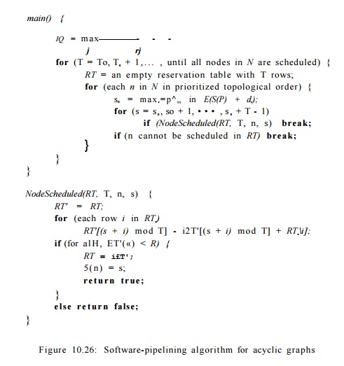
Algorithm 10.19 software pipelines acyclic data-dependence graphs. The algorithm first finds a bound on the initiation interval, To, based on the re-source requirements of the operations in the graph. It then attempts to find a software-pipelined schedule starting with To as the target initiation interval. The algorithm repeats with increasingly larger initiation intervals if it fails to find a schedule.

The algorithm uses a list-scheduling approach in each attempt. It uses a modular resource-reservation RT to keep track of the resource commitment in the steady state. Operations are scheduled in topological order so that the data dependences can always be satisfied by delaying operations. To schedule an operation, it first finds a lower bound so according to the data-dependence constraints. It then invokes NodeScheduled to check for possible resource con-flicts in the steady state. If there is a resource conflict, the algorithm tries to schedule the operation in the next clock. If the operation is found to conflict for T consecutive clocks, because of the modular nature of resource-conflict detec-tion, further attempts are guaranteed to be futile. At that point, the algorithm considers the attempt a failure, and another initiation interval is tried.

The heuristics of scheduling operations as soon as possible tends to minimize the length of the schedule for an iteration. Scheduling an instruction as early as possible, however, can lengthen the lifetimes of some variables. For example, loads of data tend to be scheduled early, sometimes long before they are used. One simple heuristic is to schedule the dependence graph backwards because there are usually more loads than stores.

8. Scheduling Cyclic Dependence Graphs

Dependence cycles complicate software pipelining significantly. When schedul-ing operations in an acyclic graph in topological order, data dependences with scheduled operations can impose only a lower bound on the placement of each operation. As a result, it is always possible to satisfy the data-dependence con-straints by delaying operations. The concept of "topological order" does not apply to cyclic graphs. In fact, given a pair of operations sharing a cycle, plac-ing one operation will impose both a lower and upper bound on the placement

of the second.

Let ni and n₂ be two operations in a dependence cycle, 5 be a software-pipeline schedule, and T be the initiation interval for the schedule. A dependence edge  m  -»•  n2     with label (6i,di)  imposes the  following  constraint  on S(ni) and   S(n2):  

Similarly, a dependence edge  ( n i , n ₂ )  with label  (5₂,d₂)  imposes constraint

A  strongly connected component  (SCC) in a graph is a set of nodes  where every node in the component can be reached by every other node in the compo-nent. Scheduling one node in an SCC will bound the time of every other node in the component both from above and from below. Transitively, if there exists a path p leading from n1 to n 2 , then

Observe that

•               Around any cycle, the sum of the S's must be positive. If it were 0 or negative, then it would say that an operation in the cycle either had to

precede itself or be executed at the same clock for all iterations.

• The schedule of operations within an iteration is the same for all iterations; that requirement is essentially the meaning of a "software pipeline." As a result, the sum of the delays (second components of edge labels in a data-dependence graph) around a cycle is a lower bound on the initiation interval T.

When we combine these two points, we see that for any feasible initiation inter-val T, the value of the right side of Equation (10.1) must be negative or zero. As a result, the strongest constraints on the placement of nodes is obtained from the simple paths — those paths that contain no cycles.

Thus, for each feasible T, computing the transitive effect of data depen-dences on each pair of nodes is equivalent to finding the length of the longest simple path from the first node to the second. Moreover, since cycles cannot increase the length of a path, we can use a simple dynamic-programming al-gorithm to find the longest paths without the "simple-path" requirement, and be sure that the resulting lengths will also be the lengths of the longest simple paths (see Exercise 10.5.7).

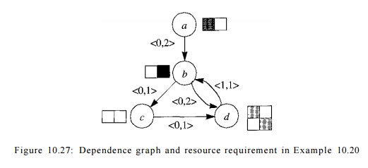
Example 10 . 20 : Figure 10.27 shows a data-dependence graph with four nodes a, b, c, d. Attached to each node is its resource-reservation table; attached to each edge is its iteration difference and delay. Assume for this example that the target machine has one unit of each kind of resource. Since there are three uses of the first resource and two of the second, the initiation interval must be no less than 3 clocks. There are two SCC's in this graph: the first is a trivial component consisting of the node a alone, and the second consists of nodes 6, c, and d. The longest cycle, b, c, d, b, has a total delay of 3 clocks connecting nodes that are 1 iteration apart. Thus, the lower bound on the initiation interval provided by data-dependence cycle constraints is also 3 clocks.

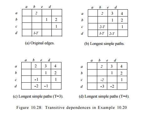
Placing any of 6, c, or d in a schedule constrains all the other nodes in the component. Let T be the initiation interval. Figure 10.28 shows the transitive dependences. Part (a) shows the delay and the iteration difference 5, for each edge. The delay is represented directly, but S is represented by "adding" to the delay the value — ST.

Figure 10.28(b) shows the length of the longest simple path between two nodes, when such a path exists; its entries are the sums of the expressions given by Fig. 10.28(a), for each edge along the path. Then, in (c) and (d), we see the expressions of (b) with the two relevant values of T, that is, 3 and 4, substituted for T. The difference between the schedule of two nodes S ( n ₂ ) - 5 ( n i ) must be no less than the value given in entry (ni, n ₂ ) in each of the tables (c) or (d), depending on the value of T chosen.

For instance, consider the entry in Fig. 10.28 for the longest (simple) path from c to 6, which is 2 — T. The longest simple path from c to b is c ->• d ->• b. The total delay is 2 along this path, and the sum of the 5's is 1, representing the fact that the iteration number must increase by 1. Since T is the time by which each iteration follows the previous, the clock at which b must be scheduled is at least 2 — T clocks after the clock at which c is scheduled. Since T is at least 3, we are really saying that b may be scheduled T — 2 clocks before c, or later than that clock, but not earlier.

Notice that considering nonsimple paths from c to b does not produce a stronger constraint. We can add to the path c —> d -» b any number of iterations of the cycle involving d and b. If we add k such cycles, we get a path length of 2 — T + k(3 — T), since the total delay along the path is 3, and the sum of the 5's is 1. Since T > 3, this length can never exceed 2 — T; i.e., the strongest lower bound on the clock of b relative to the clock of c is 2 — T, the bound we get by considering the longest simple path.

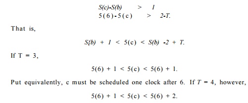
That is, c is scheduled one or two clocks after 6.

Given the all-points longest path information, we can easily compute the range where it is legal to place a node due to data dependences. We see that there is no slack in the case when T = 3, and the slack increases as T increases.

Algorithm 1 0 . 2 1 : Software pipelining.

INPUT : A machine-resource vector R = [ri,r2:...], where r« is the number of units available of the ith kind of resource, and a data-dependence graph G = (N,E). Each operation n in N is labeled with its resource-reservation table RTn] each edge e = ri1 -> n2 in E is labeled with (Se,de) indicating that n2 must execute no earlier than de clocks after node n1 from the 5eth preceding iteration.

OUTPUT : A software-pipelined schedule S and an initiation interval T.

METHOD : Execute the program in Fig. 10.29.   •

Algorithm 10.21 has a high-level structure similar to that of Algorithm 10.19, which only handles acyclic graphs. The minimum initiation interval in this case is bounded not just by resource requirements, but also by the data-dependence cycles in the graph. The graph is scheduled one strongly connected component at a time. By treating each strongly connected component as a unit, edges be-tween strongly connected components necessarily form an acyclic graph. While the top-level loop in Algorithm 10.19 schedules nodes in the graph in topological order, the top-level loop in Algorithm 10.21 schedules strongly connected com-ponents in topological order. As before, if the algorithm fails to schedule all the components, then a larger initiation interval is tried. Note that Algorithm 10.21 behaves exactly like Algorithm 10.19 if given an acyclic data-dependence graph.

Algorithm 10.21 computes two more sets of edges: E' is the set of all edges whose iteration difference is 0, E* is the all-points longest-path edges. That is,

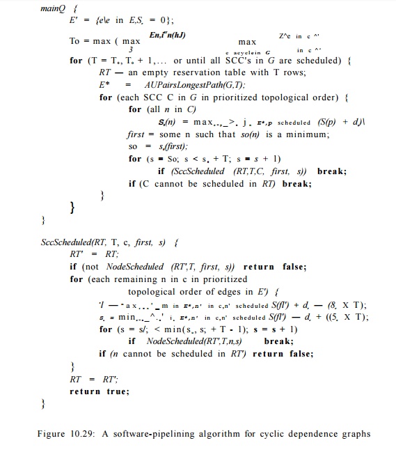
for each pair of nodes (p, n), there is an edge e in E* whose associated distance de    is the length of the longest simple path from pton, provided that there is at least one path from p to n.  E* is computed for each value of T, the initiation interval target. It is also possible to perform this computation just once with a symbolic value of T and then substitute for T in each iteration, as we did in Example 10.20.

Algorithm 10.21 uses backtracking. If it fails to schedule a SCC, it tries to reschedule the entire SCC a clock later. These scheduling attempts continue for up to T clocks. Backtracking is important because, as shown in Example 10.20, the placement of the first node in an SCC can fully dictate the schedule of all other nodes. If the schedule happens not to fit with the schedule created thus far, the attempt fails.

To schedule a SCC, the algorithm determines the earliest time each node in the component can be scheduled satisfying the transitive data dependences in E*. It then picks the one with the earliest start time as the first node to schedule. The algorithm then invokes SccScheduled to try to schedule the component at the earliest start time. The algorithm makes at most T attempts with successively greater start times. If it fails, then the algorithm tries another initiation interval.

The SccScheduled algorithm resembles Algorithm 10.19, but has three major differences.

1. The goal of SccScheduled is to schedule the strongly connected component at the given time slot s. If the first node of the strongly connected com-ponent cannot be scheduled at s, SccScheduled returns false. The main function can invoke SccScheduled again with a later time slot if that is desired.

2.         The nodes in the strongly connected component are scheduled in topolog-ical order, based on the edges in E'. Because the iteration differences on all the edges in E' are 0, these edges do not cross any iteration boundaries and cannot form cycles. (Edges that cross iteration boundaries are known as loop carried). Only loop-carried dependences place upper bounds on where operations can be scheduled. So, this scheduling order, along with the strategy of scheduling each operation as early as possible, maximizes the ranges in which subsequent nodes can be scheduled.

3.         For strongly connected components, dependences impose both a lower and upper bound on the range in which a node can be scheduled. SccSched-uled computes these ranges and uses them to further limit the scheduling attempts.

Example 10.22 : Let us apply Algorithm 10.21 to the cyclic data-dependence graph in Example 10.20. The algorithm first computes that the bound on the initiation interval for this example is 3 clocks. We note that it is not possible to meet this lower bound. When the initiation interval T is 3, the transitive dependences in Fig. 10.28 dictate that S(d) - S(b) = 2. Scheduling nodes b and d two clocks apart will produce a conflict in a modular resource-reservation table of length 3.

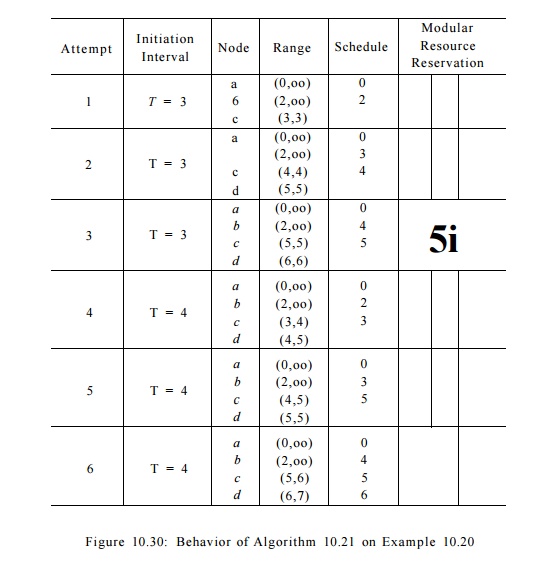
Figure 10.30 shows how Algorithm 10.21 behaves with this example. It first tries to find a schedule with a 3-clock initiation interval. The attempt starts by scheduling nodes a and b as early as possible. However, once node b is placed in clock 2, node c can only be placed at clock 3, which conflicts with the resource usage of node a. That is, a and c both need the first resource at clocks that have a remainder of 0 modulo 3.

The algorithm backtracks and tries to schedule the strongly connected com-ponent {6, c, d} a clock later. This time node b is scheduled at clock 3, and node c is scheduled successfully at clock 4. Node d, however, cannot be scheduled in clock 5. That is, both b and d need the second resource at clocks that have a remainder of 0 modulo 3. Note that it is just a coincidence that the two con-flicts discovered so far are at clocks with a remainder of 0 modulo 3; the conflict might have occurred at clocks with remainder 1 or 2 in another example.

The algorithm repeats by delaying the start of the SCC {b,c, d] by one more clock. But, as discussed earlier, this SCC can never be scheduled with an initiation interval of 3 clocks, so the attempt is bound to fail.  At this point, the algorithm gives up and tries to find a schedule with an initiation interval of 4 clocks. The algorithm eventually finds the optimal schedule on its sixth attempt.