Chapter: Compilers : Principles, Techniques, & Tools : Instruction-Level Parallelism
Code-Scheduling Constraints
Code-Scheduling Constraints
1 Data
Dependence
2 Finding
Dependences Among Memory Accesses
3 Tradeoff
Between Register Usage and Parallelism
4 Phase
Ordering Between Register Allocation and Code Scheduling
5 Control
Dependence
6 Speculative
Execution Support
7 A Basic
Machine Model
8 Exercises for
Section 10.2
Code scheduling is a form of program optimization
that applies to the machine code that is produced by the code generator. Code
scheduling is subject to three kinds of constraints:
2. Data-dependence constraints. The operations in
the optimized program must produce the same results as the corresponding ones
in the original program.
3. Resource constraints. The schedule must not
oversubscribe the resources on the machine.
These scheduling constraints guarantee that the optimized program
pro-duces the same results as the original. However, because code scheduling
changes the order in which the operations execute, the state of the memory at
any one point may not match any of the memory states in a sequential
ex-ecution. This situation is a problem if a program's execution is interrupted
by, for example, a thrown exception or a user-inserted breakpoint. Optimized
programs are therefore harder to debug. Note that this problem is not specific
to code scheduling but applies to all other optimizations, including
partial-redundancy elimination (Section 9.5) and register allocation (Section
8.8).
1.
Data Dependence
It is easy to see that if we change the execution order of two
operations that do not touch any of the same variables, we cannot possibly
affect their results. In fact, even if these two operations read the same
variable, we can still permute their execution. Only if an operation writes to
a variable read or written by another can changing their execution order alter
their results. Such pairs of operations are said to share a data dependence,
and their relative execution order must be preserved. There are three flavors
of data dependence:
1.
True
dependence: read after write. If
a write is followed by a read of the same location, the read depends on
the value written; such a dependence is known as a true dependence.
2.
Antidependence:
write after read. If a read is
followed by a write to the same location, we say that there is an
antidependence from the read to the write. The write does not depend on the
read per se, but if the write happens before the read, then the read operation
will pick up the wrong value. Antidependence is a byproduct of imperative
programming, where the same memory locations are used to store different
values. It is not a "true" dependence and potentially can be
eliminated by storing the values in different locations.
3.
Output
dependence: write after write.
Two writes to the same location share an output dependence. If the
dependence is violated, the value of the memory location written will have the
wrong value after both operations are performed.
Antidependence and output dependences are referred to as storage-related
de-pendences. These are not "true" dependences and can be
eliminated by using different locations to store different values. Note that
data dependences apply to both memory accesses and register accesses.
2. Finding Dependences Among Memory Accesses
To check if two
memory accesses share a data dependence, we only need to tell if they can refer
to the same location; we do not need to know which location is being accessed.
For example, we can tell that the two accesses *p and O p ) + 4 cannot refer to
the same location, even though we may not know what p points to. Data
dependence is generally undecidable at compile time. The compiler must assume
that operations may refer to the same location unless it can prove otherwise.
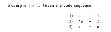
unless the compiler knows that p cannot possibly point to
a, it must conclude that the three operations need to execute serially. There
is an output depen-dence flowing from statement (1) to statement (2), and there
are two true dependences flowing from statements (1) and (2) to statement (3).
•
Data-dependence analysis is highly sensitive to the programming
language used in the program. For type-unsafe languages like C and C + + ,
where a pointer can be cast to point to any kind of object, sophisticated
analysis is necessary to prove independence between any pair of pointer-based
memory ac-cesses. Even local or global scalar variables can be accessed
indirectly unless we can prove that their addresses have not been stored
anywhere by any instruc-tion in the program. In type-safe languages like Java,
objects of different types are necessarily distinct from each other. Similarly,
local primitive variables on the stack cannot be aliased with accesses through
other names.
A correct discovery of data dependences requires a number of
different forms of analysis. We shall focus on the major questions that must be
resolved if the compiler is to detect all the dependences that exist in a
program, and how to use this information in code scheduling. Later chapters
show how these analyses are performed.
Array Data - Dependence Analysis
Array data dependence
is the problem of disambiguating between the values of indexes in array-element
accesses. For example, the loop
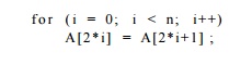
copies odd elements in the array A to the even elements
just preceding them. Because all the read and written locations in the loop are
distinct from each other, there are no dependences between the accesses, and
all the iterations in the loop can execute in parallel. Array data-dependence
analysis, often referred to simply as data-dependence analysis, is very
important for the optimization of numerical applications. This topic will be
discussed in detail in Section 11.6.
Pointer - Alias Analysis
We say that two pointers are aliased if they can refer to
the same object. Pointer-alias analysis is difficult because there are many
potentially aliased pointers in a program, and they can each point to an
unbounded number of dynamic objects over time. To get any precision,
pointer-alias analysis must be applied across all the functions in a program.
This topic is discussed starting in Section 12.4.
Interprocedural Analysis
For languages that pass parameters by reference, interprocedural
analysis is needed to determine if the same variable is passed as two or more
different arguments. Such aliases can create dependences between seemingly
distinct parameters. Similarly, global variables can be used as parameters and
thus create dependences between parameter accesses and global variable
accesses. Interprocedural analysis, discussed in Chapter 12, is necessary to
determine these aliases.
3. Tradeoff Between Register Usage and Parallelism
In this chapter we shall assume that the machine-independent
intermediate rep-resentation of the source program uses an unbounded number of pseudoregisters
to represent variables that can be allocated to registers. These variables
include scalar variables in the source program that cannot be referred to by
any other names, as well as temporary variables that are generated by the
compiler to hold the partial results in expressions. Unlike memory locations,
registers are uniquely named. Thus precise data-dependence constraints can be
generated for register accesses easily.
The unbounded number
of pseudoregisters used in the intermediate repre-sentation must eventually be
mapped to the small number of physical registers available on the target
machine. Mapping several pseudoregisters to the same physical register has the
unfortunate side effect of creating artificial storage dependences that
constrain instruction-level parallelism. Conversely, executing instructions in
parallel creates the need for more storage to hold the values being computed
simultaneously. Thus, the goal of minimizing the number of registers used
conflicts directly with the goal of maximizing instruction-level parallelism.
Examples 10.2 and 10.3 below illustrate this classic trade-off between storage
and parallelism.
Hardware Register Renaming
Instruction-level
parallelism was first used in computer architectures as a means to speed up
ordinary sequential machine code. Compilers at the time were not aware of the
instruction-level parallelism in the machine and were designed to optimize the
use of registers. They deliberately reordered instructions to minimize the
number of registers used, and as a result, also minimized the amount of
parallelism available. Example 10.3
illustrates how minimizing register usage in the computation of expression
trees also limits its parallelism.
There was so little
parallelism left in the sequential code that computer architects invented
the concept of
hardware register renaming to undo the effects of register optimization
in compilers. Hardware register renaming
dynamically changes the assignment of registers as the program runs. It interprets the machine code, stores values
intended for the same register in different internal registers, and updates all
their uses to refer to the right registers accordingly.
Since the artificial
register-dependence constraints were introduced by the compiler in the first
place, they can be eliminated by using a register-allocation algorithm that is
cognizant of instruction-level paral-lelism. Hardware register renaming is
still useful in the case when a ma-chine's instruction set can only refer to a
small number of registers. This capability allows an implementation of the
architecture to map the small number of architectural registers in the code to
a much larger number of internal registers dynamically.
Example 10.2 : The code below copies the values of variables
in locations a and c to variables in locations b and d, respectively, using
pseudoregisters tl and t2.
LD t l , a
ST b , t l
LD t2, c
ST d, t2
/ / t l = a
/ / b = t l
/ / t2 = c
/ / d = t2
If all the memory
locations accessed are known to be distinct from each other, then the copies
can proceed in parallel. However, if tl and t2 are assigned the same register
so as to minimize the number of registers used, the copies are necessarily
serialized. •
Example 10.3 :
Traditional register-allocation techniques aim to minimize the number of
registers used when performing a computation. Consider the expression
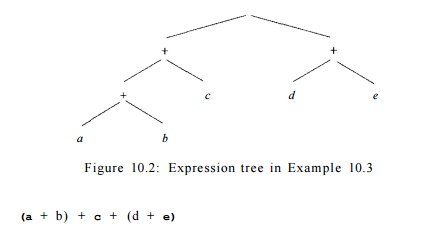
shown as a syntax
tree in Fig. 10.2. It is possible to perform this computation using three
registers, as illustrated by the machine code in Fig. 10.3.
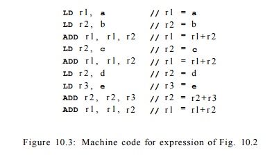
The reuse of registers, however, serializes the computation. The
only oper-ations allowed to execute in parallel are the loads of the values in
locations a and b, and the loads of the values in locations d
and e. It thus takes a total of 7 steps to complete the
computation in parallel.
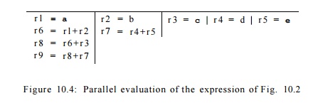
Had we used different
registers for every partial sum, the expression could be evaluated in 4 steps,
which is the height of the expression tree in Fig. 10.2. The parallel
computation is suggested by Fig. 10.4.
4. Phase Ordering Between Register Allocation and Code Scheduling
If registers are allocated before scheduling, the resulting code
tends to have many storage dependences that limit code scheduling. On the other
hand, if code is scheduled before register allocation, the schedule created may
require so many registers that register
spilling (storing the contents
of a register in a memory location, so the register can be used for some
other purpose) may negate the advantages of instruction-level parallelism.
Should a compiler allo-cate registers first before it schedules the code? Or
should it be the other way round? Or, do we need to address these two problems
at the same time?
To answer the questions above, we must consider the
characteristics of the programs being compiled. Many nonnumeric applications do
not have that much available parallelism. It suffices to dedicate a small
number of registers for holding temporary results in expressions. We can first
apply a coloring algorithm, as in Section 8.8.4, to allocate registers for all the
nontemporary variables, then schedule the code, and finally assign registers to
the temporary variables.
This approach does
not work for numeric applications where there are many more large expressions.
We can use a hierarchical approach where code is op-timized inside out,
starting with the innermost loops. Instructions are first scheduled assuming
that every pseudoregister will be allocated its own physical register. Register
allocation is applied after scheduling and spill code is added where necessary,
and the code is then rescheduled. This process is repeated for the code in the
outer loops. When several inner loops are considered together in a common outer
loop, the same variable may have been assigned different registers. We can
change the register assignment to avoid having to copy the values from one
register to another. In Section 10.5, we shall discuss the in-teraction between
register allocation and scheduling further in the context of a specific
scheduling algorithm.
5. Control
Dependence
Scheduling operations within a basic block is relatively easy
because all the instructions are guaranteed to execute once control flow
reaches the beginning of the block. Instructions in a basic block can be
reordered arbitrarily, as long as all the data dependences are satisfied.
Unfortunately, basic blocks, especially in nonnumeric programs, are typically
very small; on average, there are only about five instructions in a basic
block. In addition, operations in the same block are often highly related and thus
have little parallelism. Exploiting parallelism across basic blocks is
therefore crucial.
An optimized program
must execute all the operations in the original pro-gram. It can execute more
instructions than the original, as long as the extra instructions do not change
what the program does. Why would executing extra instructions speed up a
program's execution? If we know that an instruction is likely to be executed,
and an idle resource is available to perform the opera-tion "for
free," we can execute the instruction speculatively. The program
runs faster when the speculation turns out to be correct.
An instruction
n is said to be control-dependent on instruction
i2 if the outcome of i2 determines whether h is to be executed. The
notion of control dependence corresponds to the concept of nesting levels in
block-structured programs. Specifically, in the if-else statement
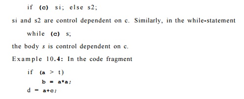
the statements b = a*a and d = a+c have no data dependence with any other part of
the fragment. The statement b = a*a depends on the comparison a > t. The
statement d = a+c, however, does not depend on the comparison and
can be executed any time. Assuming that the multiplication a * a does
not cause any side effects, it can be performed speculatively, as long as b
is written only after a is found to be greater than t. •
6. Speculative Execution Support
Memory loads are one type of instruction that can benefit greatly
from specula-tive execution. Memory loads are quite common, of course. They
have relatively long execution latencies, addresses used in the loads are
commonly available in advance, and the result can be stored in a new temporary
variable without destroying the value of any other variable. Unfortunately,
memory loads can raise exceptions if their addresses are illegal, so
speculatively accessing illegal addresses may cause a correct program to halt
unexpectedly. Besides, mispre-dicted memory loads can cause extra cache misses
and page faults, which are extremely costly.
Example 10.5
: In the fragment
if (p
!= n u l l )
q = *P;
dereferencing p speculatively will cause this correct
program to halt in error if p is null .
Many high-performance
processors provide special features to support spec-ulative memory accesses. We
mention the most important ones next.
Prefetching
The prefetch instruction was invented to bring data from
memory to the cache before it is used. A prefetch instruction indicates
to the processor that the program is likely to use a particular memory word in
the near future. If the location specified is invalid or if accessing it causes
a page fault, the processor can simply ignore the operation. Otherwise, the
processor will bring the data from memory to the cache if it is not already
there.
Poison Bits
Another architectural feature called poison bits was
invented to allow specu-lative load of data from memory into the register file.
Each register on the machine is augmented with a poison bit. If illegal
memory is accessed or the accessed page is not in memory, the processor does
not raise the exception im-mediately but instead just sets the poison bit of
the destination register. An exception is raised only if the contents of the
register with a marked poison bit are used.
Predicated Execution
Because branches are expensive, and mispredicted branches are even
more so (see Section 10.1), predicated instructions were invented to
reduce the number of branches in a program. A predicated instruction is like a
normal instruction but has an extra predicate operand to guard its execution;
the instruction is executed only if the predicate is found to be true.
As an example, a
conditional move instruction CMOVZ
R2,R3,R1 has the semantics
that the contents of register R3 are moved to register R2 only if register Rl is zero. Code such as
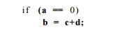
can be implemented
with two machine instructions, assuming that a, b, c, and d are
allocated to registers Rl,
R2, R4, R5, respectively, as follows:

This conversion replaces a series of instructions sharing a
control dependence with instructions sharing only data dependences. These
instructions can then be combined with adjacent basic blocks to create a larger
basic block. More importantly, with this code, the processor does not have a
chance to mispredict, thus guaranteeing that the instruction pipeline will run
smoothly.
Predicated execution
does come with a cost. Predicated instructions are fetched and decoded, even
though they may not be executed in the end. Static schedulers must reserve all
the resources needed for their execution and ensure
Dynamically Scheduled
Machines
The instruction set of a statically scheduled machine explicitly
defines what can execute in parallel. However, recall from Section 10.1.2 that
some ma-chine architectures allow the decision to be made at run time about
what can be executed in parallel. With dynamic scheduling, the same machine
code can be run on different members of the same family (machines that
implement the same instruction set) that have varying amounts of
parallel-execution support. In fact, machine-code compatibility is one of the
major advantages of dynamically scheduled machines.
Static schedulers, implemented in the compiler by software, can
help dynamic schedulers (implemented in the machine's hardware) better utilize
machine resources. To build a static scheduler for a dynamically sched-uled
machine, we can use almost the same scheduling algorithm as for statically
scheduled machines except that no - op instructions left in the schedule need
not be generated explicitly. The matter is discussed further in Section 10.4.7.
that all the potential data dependences are satisfied. Predicated
execution should not be used aggressively unless the machine has many more
resources than can possibly be used otherwise.
7. A Basic Machine Model
Many machines can be represented using the following simple model.
A machine M = {R,T), consists of:
1.
A set of
operation types T, such as loads, stores, arithmetic operations, and so on.
2.
A vector R =
[n, r2,... ] representing hardware resources, where r« is the number of
units available of the ith kind of resource. Examples of typical
resource types include: memory access units, ALU's, and floating-point
functional units.
Each operation has a set of input operands, a set of output
operands, and a resource requirement. Associated with each input operand is an
input latency indicating when the input value must be available (relative to
the start of the operation). Typical input operands have zero latency, meaning
that the values are needed immediately, at the clock when the operation is
issued. Similarly, associated with each output operand is an output latency,
which indicates when the result is available, relative to the start of the
operation.
Resource usage for each machine operation type t is modeled
by a two-dimensional resource-reservation table, RTt. The width of the table is the number of kinds of
resources in the machine, and its length is the duration over which resources
are used by the operation. Entry RTt[i,j] is the number of units of the j t h resource used
by an operation of type t, i clocks after it is issued. For notational
simplicity, we assume RTt[i,j] = 0 if i refers to a nonex-istent entry in the table (i.e., i
is greater than the number of clocks it takes to execute the operation). Of
course, for any t, i, and j, RTt[i,j] must be less than or equal to R[j], the
number of resources of type j that the machine has.
Typical machine
operations occupy only one unit of resource at the time an operation is issued.
Some operations may use more than one functional unit. For example, a
multiply-and-add operation may use a multiplier in the first clock and an adder
in the second. Some operations, such as a divide, may need to occupy a resource
for several clocks. Fully pipelined operations are those that can be
issued every clock, even though their results are not available until some
number of clocks later. We need not model the resources of every stage of a
pipeline explicitly; one single unit to represent the first stage will do. Any
operation occupying the first stage of a pipeline is guaranteed the right to
proceed to subsequent stages in subsequent clocks.
1) a = b
2) c = d
3) b = c
4) d = a
5) c = d
6) a = b
Figure 10.5: A sequence of assignments exhibiting data
dependences
8. Exercises for Section 10.2
Exercise 1 0 . 2 . 1 : The assignments in Fig. 10.5 have
certain dependences. For each of the following pairs of statements, classify
the dependence as (i) true de-pendence, (n) antidependence, (Hi)
output dependence, or (iv) no dependence (i.e., the instructions can
appear in either order):
a)
Statements (1)
and (4).
b)
Statements (3)
and (5).
c)
Statements (1)
and (6).
d)
Statements (3)
and (6).
e)
Statements (4)
and (6).
Exercise 10 . 2 . Evaluate the expression ((u+v) + (w+x)) + (y+z)
exactly as do not 2: parenthesized (i.e., use the commutative or associative
laws to reorder the additions). Give register-level machine code to provide the
maximum possible parallelism.
Exercise 10 . 2 . 3 : Repeat
Exercise 10.2.2 for the following expressions:
a) (u + (v + (w + x))^j + (y + z).
b) (u + (v + w)) + (x + {y + z)).
If instead of maximizing the parallelism, we minimized the number
of registers, how many steps would the computation take? How many steps do we
save by using maximal parallelism?
Exercise 1 0 . 2 . 4 : The expression of Exercise 10.2.2 can be
executed by the sequence of instructions shown in Fig. 10.6. If we have
as much parallelism as we need, how many steps are needed to execute the
instructions?
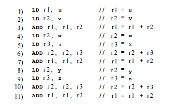
Figure 10.6: Minimal-register implementation of an
arithmetic expression
Exercise 1 0 . 2 . 5 : Translate the code fragment discussed in Example 10.4, using
the CM0VZ conditional copy instruction of Section 10.2.6. What are the
data dependences in your machine code?
Related Topics