Basic-Block Scheduling

Basic-Block Scheduling

1 Data-Dependence Graphs

2 List Scheduling of Basic Blocks

3 Prioritized Topological Orders

4 Exercises for Section 10.3

We are now ready to start talking about code-scheduling algorithms. We start with the easiest problem: scheduling operations in a basic block consisting of machine instructions. Solving this problem optimally is NP-complete. But in practice, a typical basic block has only a small number of highly constrained operations, so simple scheduling techniques suffice. We shall introduce a simple but highly effective algorithm, called list scheduling, for this problem.

1. Data-Dependence Graphs

We represent each basic block of machine instructions by a data-dependence graph, G = (N,E), having a set of nodes iV representing the operations in the machine instructions in the block and a set of directed edges E representing the data-dependence constraints among the operations. The nodes and edges of G are constructed as follows:

1. Each operation n in N has a resource-reservation table RT_n, whose value is simply the resource-reservation table associated with the operation type of n.

2. Each edge e in E is labeled with delay d_e indicating that the destination node must be issued no earlier than d_e clocks after the source node is issued. Suppose operation n± is followed by operation n₂, and the same location is accessed by both, with latencies l1 and l₂ respectively. That is, the location's value is produced l1 clocks after the first instruction begins, and the value is needed by the second instruction l₂ clocks after that instruction begins (note — 1 and l₂ = 0 is typical). Then, there is an edge n1 -» n₂ in E labeled with delay l1 — l₂.

Example 1 0 . 6 : Consider a simple machine that can execute two operations every clock. The first must be either a branch operation or an ALU operation of the form:

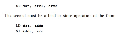
The load operation (LD) is fully pipelined and takes two clocks. However, a load can be followed immediately by a store ST that writes to the memory location read. All other operations complete in one clock.

Shown in Fig. 10.7 is the dependence graph of an example of a basic block and its resources requirement. We might imagine that Rl is a stack pointer, used to access data on the stack with offsets such as 0 or 12. The first instruction loads register R2, and the value loaded is not available until two clocks later. This observation explains the label 2 on the edges from the first instruction to the second and fifth instructions, each of which needs the value of R2. Similarly, there is a delay of 2 on the edge from the third instruction to the fourth; the value loaded into R3 is needed by the fourth instruction, and not available until two clocks after the third begins.

Since we do not know how the values of Rl and R7 relate, we have to consider the possibility that an address like 8 (Rl) is the same as the address 0 (R7). That

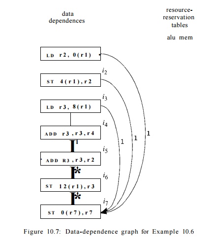
is, the last instruction may be storing into the same address that the third instruction loads from. The machine model we are using allows us to store into a location one clock after we load from that location, even though the value to be loaded will not appear in a register until one clock later. This observation explains the label 1 on the edge from the third instruction to the last. The same reasoning explains the edges and labels from the first instruction to the last. The other edges with label 1 are explained by a dependence or possible dependence conditioned on the value of R7. •

2. List Scheduling of Basic Blocks

The simplest approach to scheduling basic blocks involves visiting each node of the data-dependence graph in "prioritized topological order." Since there can be no cycles in a data-dependence graph, there is always at least one topological order for the nodes. However, among the possible topological orders, some may be preferable to others. We discuss in Section 10.3.3 some of the strategies for picking a topological order, but for the moment, we just assume that there is some algorithm for picking a preferred order.

Pictorial Resource-Reservation Tables

It is frequently useful to visualize a resource-reservation table for an oper-ation by a grid of solid and open squares. Each column corresponds to one of the resources of the machine, and each row corresponds to one of the clocks during which the operation executes. Assuming that the operation never needs more than one unit of any one resource, we may represent l's by solid squares, and O's by open squares. In addition, if the operation is fully pipelined, then we only need to indicate the resources used at the first row, and the resource-reservation table becomes a single row.

This representation is used, for instance, in Example 10.6. In Fig. 10.7 we see resource-reservation tables as rows. The two addition operations require the "alu" resource, while the loads and stores require the "mem" resource.

The list-scheduling algorithm we shall describe next visits the nodes in the chosen prioritized topological order. The nodes may or may not wind up being scheduled in the same order as they are visited. But the instructions are placed in the schedule as early as possible, so there is a tendency for instructions to be scheduled in approximately the order visited.

In more detail, the algorithm computes the earliest time slot in which each node can be executed, according to its data-dependence constraints with the previously scheduled nodes. Next, the resources needed by the node are checked against a resource-reservation table that collects all the resources committed so far. The node is scheduled in the earliest time slot that has sufficient resources.

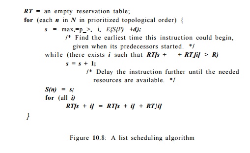
Algorithm 1 0 . 7 : List scheduling a basic block.

INPUT : A machine-resource vector R — [ r i , r 2 , . . . ] , where r« is the number of units available of the ith kind of resource, and a data-dependence graph G — (N, E). Each operation n in N is labeled with its resource-reservation table RTn; each edge e = ni —> n2 in E is labeled with de indicating that n2 must execute no earlier than de clocks after m.

OUTPUT : A schedule S that maps the operations in N into time slots in which the operations can be initiated satisfying all the data and resources constraints.

METHOD : Execute the program in Fig. 10.8. A discussion of what the "prior-itized topological order" might be follows in Section 10.3.3.

3. Prioritized Topological Orders

List scheduling does not backtrack; it schedules each node once and only once. It uses a heuristic priority function to choose among the nodes that are ready to be scheduled next. Here are some observations about possible prioritized orderings of the nodes:

• Without resource constraints, the shortest schedule is given by the critical path, the longest path through the data-dependence graph. A metric  useful as a priority function is the height of the node, which is the length of a longest path in the graph originating from the node.

•  On the other  hand, if all operations  are independent,  then the length of the schedule is constrained by the resources available. The critical resource is the one with the largest ratio of uses to the number of units of that resource available. Operations using more critical resources may be given higher priority.

• Finally, we can use the source ordering to break ties between operations; the operation that shows up earlier in the source program should be sched-uled first.

Example 10.8 : For the data-dependence graph in Fig. 10.7, the critical path, including the time to execute the last instruction, is 6 clocks. That is, the critical path is the last five nodes, from the load of R3 to the store of R7. The total of the delays on the edges along this path is 5, to which we add 1 for the clock needed for the last instruction.

Using the height as the priority function, Algorithm 10.7 finds an optimal schedule as shown in Fig. 10.9. Notice that we schedule the load of R3 first, since it has the greatest height. The add of R3 and R4 has the resources to be

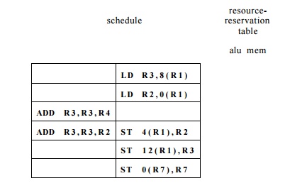
Figure 10.9:  Result of applying list scheduling to the example in Fig. 10.7 scheduled at the second clock, but the delay of 2 for a load forces us to wait until the third clock to schedule this add. That is, we cannot be sure that R3 will have its needed value until the beginning of clock 3.

4. Exercises for Section 10.3

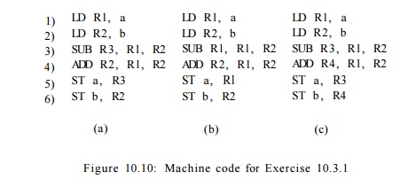
Exercise 10. 3 . 1 : For each of the code fragments of Fig. 10.10, draw the data-dependence graph.

Exercise 10.3.2 : Assume a machine with one ALU resource (for the ADD and SUB operations) and one MEM resource (for the LD and ST operations). Assume that all operations require one clock, except for the LD, which requires two. However, as in Example 10.6, a ST on the same memory location can commence one clock after a LD on that location commences. Find a shortest schedule for each of the fragments in Fig. 10.10.

Exercise 1 0 . 3 . 3 :       Repeat        Exercise 10.3.2     assuming:

i. The machine has one ALU resource and two MEM resources.

ii. The machine has two ALU resources and one MEM resource.

iii.  The machine has two ALU resources and two MEM resources.

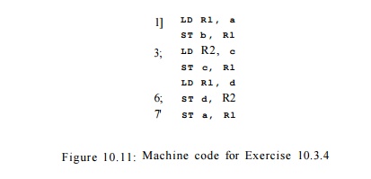
Exercise 1 0 . 3 . 4: Assuming the machine model of Example 10.6 (as in Exer-cise 10.3.2):

a)  Draw the data dependence graph for the code of Fig. 10.11.

b)  What are all the critical paths in your graph from part (a)?

 c) Assuming unlimited MEM resources, what are all the possible schedules for the seven instructions?