Harmonic Holes for Free Fields

Harmonic Holes for Free Fields

Solutions for harmonic holes from the basic equations presented in the previ-ous section are possible, in theory, for any elasticity field where the “opening” (unloaded, loaded, or an inclusion) is far enough from any other boundary so as to avoid significant interaction effects. Here we will concentrate on the results* for self-sustaining biaxial and gradient fields because of their funda-mental interest and immediate applicability to design.

The basic equations are derived with general boundary loading and dis-placement functions F(σ) and D(σ), and the significance of this capability to control the harmonic shape for particular applications should be emphasized. Practically any combination of internal tractions and displacements expressed as a function of an angular coordinate, θ, could be examined as, for example, prestress with expandable liners or “shrink fitting.” However, to emphasize the basic idea and because so little work has been done on the inverse prob-lem, harmonic shapes will be derived for holes with uniform loading and for rigid inclusions.

Harmonic Holes for Biaxial Fields

Since the biaxial field is so commonly encountered in structural mechanics, it is selected first to illustrate the application of the general functional equation. In addition, a uniformly distributed normal traction of magnitude P (positive if tension) applied to the unknown hole boundary is also included. Thus the boundary loading function is

where P is zero for the unloaded hole.

For the plane problem, consider the biaxial free field specified by the prin-cipal stresses N1, N2, which have constant magnitude and direction at every point in the plane and where it will always be assumed that the direction of N1 coincides with the x-axis and that |N1| >= |N2|. For these conditions

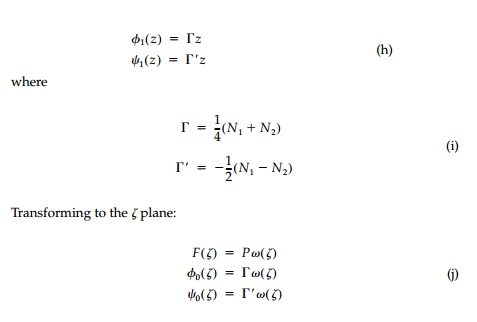
Finally, substituting these expressions into the general integral equation and combining similar terms, one obtains

Substituting, the coefficient a1 can be expressed in terms of the principal stresses as

Thus the mapping function whose boundary value describes the geometry of the harmonic hole for a biaxial field with uniform boundary loading is

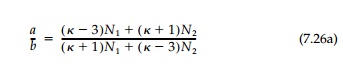
In the z-plane the boundary value of this mapping function describes an elliptic hole with major axis, a, oriented parallel to the direction of the major prin-cipal stress N1, and where the ratio of the major to minor axes of the ellipse is

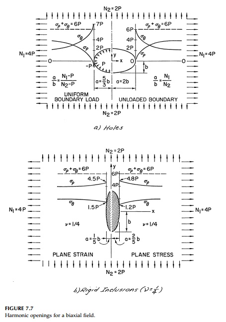
Harmonic holes with stresses along the x-axis for a particular biaxial field are shown in Figure 7.7a.

Conditions to ensure the existence of a harmonic hole shape in a biaxial field correspond to a breakdown in the conformality of () which, in turn, coincide with physical conditions on the original stress field. Considering the first derivative of the mapping function on the boundary,

the conformality of ω(σ) breaks down when a1 =   +- 1. However, if the direction of N1 is to be parallel with the direction of the major axis of the ellipse, as has been specified, a1 can only vary between 0 and + 1. Obviously, if a1  = 0, a cir-cular hole is the harmonic shape; and this occurs when N1=N2 regardless of the value of P. For a1 =+ 1, the harmonic hole is a slit parallel to the direction of N1. In the case of an unloaded hole (i.e., P = 0), the limitations on the values for the coefficient a1, establish the following limitation on the field:

This relationship is satisfied only if N1 and N2 have the same sign (i.e., both tension or both compression). In the case of a uniformly loaded hole

This relationship is satisfied when N1 is positive (i.e., tension) only if N2 <=P and when N1 is negative (i.e., compression) only if N2  P. It is helpful to note that these limitations on the type of biaxial field for which a harmonic hole exists may be more easily visualized by realizing that the ratio a/b in Equation (7.25) must always be greater than or equal to one.

At the other extreme of a rigid inclusion, the harmonic shape can be found from Equation (7.23b) following an analogous procedure. Substituting, Equation (7.24) becomes

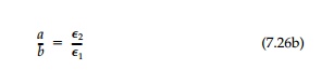
Thus, the rigid harmonic inclusion is an ellipse of arbitrary size with the ratio of major to minor axes:

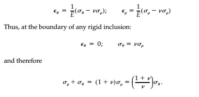
or, in terms of principal normal strains, simply

the variable a coinciding with the x-axis. In an isotropic field where N1=N2 the shape, as expected, is a circle.

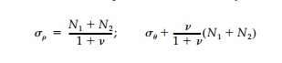
The stresses on the boundary of any rigid inclusion are

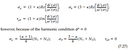
As can be seen, harmonic inclusions not only give the required condition  σθ = N1 + N2 at the interface, but also no shears so that, in fact, the contact stresses are principal with no tendency for slip to occur at the interface.

To demonstrate these results, the same test case N1 = 2N2 = 4P with v =1/4 is shown in Figure 7.7b for both plane stress and plane strain. Both harmonic holes and harmonic inclusions are ellipses oriented with the principal stresses but in opposite directions. The unloaded harmonic hole has a ratio of the axes proportional to the ratio of the original principal stresses while this ratio for the elliptic harmonic inclusion is inversely proportional to the original princi-pal strains (irrespective of the planar condition).

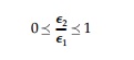
For the rigid inclusion, the condition for existence is similar to that for holes in that a/b > 0 and therefore it can exist only when

It is clear that holes that are harmonic must produce minimum stress concen-tration in constant fields since maximums and minimums in Laplacian fields must occur on the boundary. It can now be shown that the same is true for a rigid harmonic inclusion. For example, in plane stress the in-plane normal strains are given by:

But the minimum value possible for the first invariant in a constant field is simply N1+ N2 so the minimum stresses possible on the boundary are:

which are in fact, those for the harmonic inclusion [Equation (7.27)]. The proof for plane strain is similar. Although the standard uniqueness theorems of elasticity do not apply directly to the “inverse problem,” it is hard to con-ceive of other shapes that might fulfill the harmonic design requirement for a given original stress field since this would be comparable to finding two different shapes that have precisely the same value of stress or displacement at every point on the boundary. Again comparing the two “extreme” alterna-tives of holes and rigid inclusions, it seems, from Figure 7.7 that a rigid inclu-sion is somewhat closer than an unloaded hole to the absolute optimum of a neutral hole with no stress concentration whatsoever. Comparing each har-monic shape for the test case N1 = 2N2, = 1/4, to the corresponding circular shape, the stress concentration factor is reduced from 2.5 to 1.5 for an unloaded hole and from 1.56 to 1.2 for a rigid inclusion in plane stress. In either case, the practical benefits that accrue from using harmonic shapes are important.

Harmonic Holes for Gradient Fields

Using the complex-variable representation of the plane theory of elasticity, it has been possible to invert the standard problems of classical elasticity to solve for the geometry of a hole that does not anywhere perturb the first invariant of the original free field. This design criterion and the resulting shapes are termed “harmonic” not only because the first invariant, which is harmonic, remains everywhere unchanged, but also because all perturba-tions of the original stress�'strain field are harmonic as well. For a constant field the harmonic ellipse does produce constant boundary stresses and a minimum stress concentration and it is postulated that such harmonic shapes are, in fact, “optimum” in that they produce minimum stress concentrations in any field for which they exist.

In theory at least, the harmonic field condition, Equation (7.20), and the resulting boundary integral Equations (7.23) apply to any field. The only unknown in these equations is the harmonic hole geometry ω(σ), which is the boundary value of the conformal mapping z = ω(ζ) from the exterior |ζ| =1 of the unit circle in the ζ- plane. The complex potentials ϕ0(σ) and Ψ(σ), which define the original free field, and F(σ) and D(σ), which describe the boundary loading or deflection are always known functions of ω(σ). In these terms, σ (no subscript) is the value of ξ =p ei^θ on the boundary of the unit cir-cular hole γ with center at the origin (i.e., σ = eiθ).

A solution of this equation for  ω(σ) therefore determines the harmonic hole shape. In addition, it should be reemphasized that the equation admits great generality in that one may obtain solutions for either constant or nonconstant fields with either constant or nonconstant boundary loads.

Consider the simple case of a linear gradient field (e.g., bending) acting within a region large in comparison with the size of a hole to be cut. Super-imposing on this field an isotropic field, the resulting components of the com-bined field in the absence of a hole are

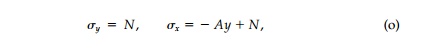
where A is a real constant that determines the slope of the linear field and N is the magnitude of the isotropic field component. The fact that this stress field is unbounded at infinity causes no particular difficulty since one need only consider a sufficiently large finite region in which all stresses are bounded.

For this combined field with a uniform pressure “P” (positive if tension) on the hole boundary:

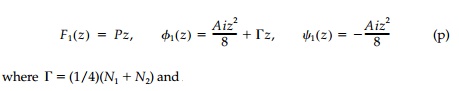
N1, N2 are the principal stresses. Transforming these equations to the ξ-plane they become

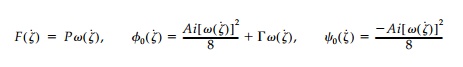
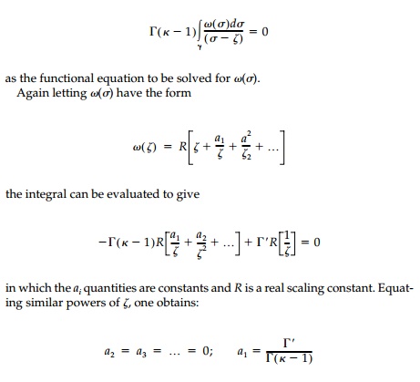
Finally, substituting the foregoing expressions into the harmonic hole equa-tion and combining terms one obtains as the functional equation to be solved for ω(σ):

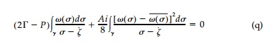
It is important to note that unlike integral equations encountered in the solution of the standard elasticity problem where the mapping function is known, Equation (q) expresses the condition that must be satisfied by the boundary value of the unknown mapping function. Since it is the boundary value of the final mapping function that must satisfy Equation (q), it is only necessary that functional representation of ω(σ) be shown as a gen-eral rational polynomial containing both negative and positive powers of

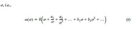
In this equation R is a real scaling constant and the a’s and b’s are complex constants. As can be seen, such an expression allows a far more concise representation of the hole geometry than could be obtained if the positive powers of  σ >2 were omitted and, in fact, if these positive powers of σ are not included, a closed-form polynomial solution cannot be obtained.

Substituting Equation (r) into Equation (q) and evaluating, one can show that a solution exists when

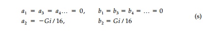
Here, G is a nondimensional parameter called the “gradient field strength,” which relates the relative strength of the original field components (A,�'), the half depth of the hole (R), and the boundary loading

In the present case of a gradient superimposed on an isotropic field, G = 2AR/(N - P). Thus the boundary value of the mapping function that describes the shape of the harmonic hole for an isotropic field with superimposed linear gradient and uniform boundary loading is

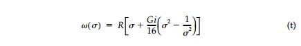
This harmonic hole shape is called the “deloid.” When the point σ in Equation (t) describes the unit circle γ, the point (x, y) describes the deloid in the z-plane the parametric representation of which is

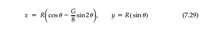
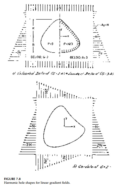
The geometry of a deloid with an unloaded boundary for an original stress field of G = 2.0 and a deloid in the same original stress field, but with a uni-form boundary loading that results in a G = 3.0 is shown in Figure 7.8a.

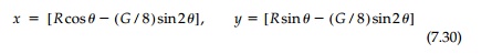
Following the same procedure for a stress field where both principal stresses vary linearly, the “cardeloid” can be obtained with the parametric representation:

Using Equation (t) the range of values of G for which ω(σ) presents a con-formal transformation can be obtained. This range is the same for both the deloid and cardeloid and is simply |G|<4.0. In the case of the unloaded hole (i.e., P = 0) this condition establishes the following limitation on the stress field and hole size:

which is physically satisfied only if the entire hole boundary occupies a region in the original stress field where the first invariant (or mean stress) has the same sign.

While it has been postulated that harmonic holes are also optimum in that they produce minimum values of stress concentration for any hole shape in any free field for which they exist, this postulate has only been proven for the constant free-field. Nonetheless one can obtain an idea of the extent to which harmonic holes can reduce stress concentrations in nonconstant fields by com-paring the stresses on the boundary of an unloaded harmonic hole to those for a circular hole most commonly encountered in practice.

For example, Figure 7.9 shows the boundary values of the tangential normal stress τ_θ nondimensionalized by the isotropic field stress N, for the deloid G= 3.0 and a circular hole of the same size in the same position. It is clear that the

deloid has not only significantly reduced the maximum stress, but it has also significantly reduced the total variation of stress around the hole boundary.

In the next two sections we will go on to the question of the neutral hole where both the shape and the properties of reinforcement to eliminate all stress concentration are presented for the same simple free fields discussed here for unlined harmonic holes. However, the essence of inverting elastic analysis to a design orientation should not be lost in the details of a particular solution. Since the inverse problem in elasticity has received so little attention and less “theoretical” treatment, time has been spent here on formulating it properly, deriving some basic equations, and emphasizing the overriding importance and effects of the design condition rather than generating solu-tions for many specific design situations. Essentially, any initial field for which the stress function is known can now be investigated and shapes derived of practical interest and importance. There are also a myriad of pos-sibilities and directions for further basic study. The exterior problem, ques-tions of existence and uniqueness, nonhomogeneous or nonisotropic materials, energy formulations, other design conditions, and related prob-lems in other areas of applied science are a few of the obvious possibilities.