Functions in OpenOffice Calc

Functions in OpenOffice Calc

Introduction

A function is a predefined calculation entered in a cell to help to analyze or manipulate data in a spreadsheet. These functions simplify help to create the formulas needed to get the expected results. Formulae are equations using numbers and variables to get a result. In a spreadsheet, the variables are cell locations that hold the data needed for the equation to be completed. Open Office Calc includes over 350 functions to analyze and reference data. Many of these functions are used for working on numbers, dates, times, and text.

Familiarization with the categories of functions

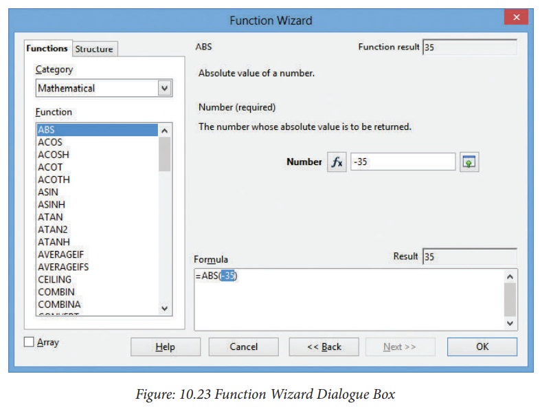
The most commonly used feature input method is built-in functions.the Function Wizard. To open the Function Wizard can be opened through , the menu choose Insert→ Function or using the shortcut key press Ctrl+F2.

1. Once open, Select a category of functions to shorten the list, then scroll down through the named functions and select the required one.

2. When you select a function its description appears on the right-hand side of the dialog. Double-click on the required function.

3. The Wizard now displays a textbox where you can enter data manually in text boxes and the result will be displayed in the Result text box

Working with the functions in Mathematical and Statistical Category

1. - Mathematical functions under Mathematical Category:

Various Mathematical function are readily available under Mathematical category for mathematical calculations.

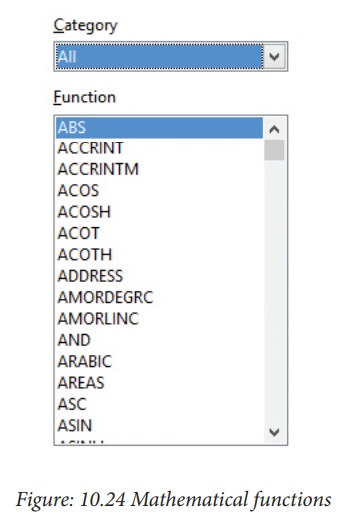
Few mathematical functions are listed below.

ABS (Number/Cell Address)

Number/ Cell Address is the value whose absolute value is to be calculated. The absolute value of a number is its value without +/- sign.

Example

=ABS (-76) returns 76, =ABS (74) returns 7, =ABS (0) returns 0.

ACOS (Number/Cell Address)

This function returns the inverse trigonometric cosine of Number that is the angle (in radians) whose cosine is Number. The angle returned is in the range 0.0 to +PI. To return the angle in degrees, use the DEGREES function.

Example

=ACOS (-1) returns 3.14159265358979 (PI radians)

=DEGREES (ACOS(0.5)) returns 60. The cosine of 60 degrees is 0.5.

ACOSH (Number/Cell Address)

This function returns the inverse hyperbolic cosine of Number, whose hyperbolic cosine is Number. Number must be greater than or equal to +1.0.

Example

=ACOSH(1) returns 0, =ACOSH(COSH(4)) returns 4.

ACOT(Number/Cell Address)

This function returns the inverse trigonometric cotangent of Number i.e. the angle (in radians) whose cotangent is Number. The angle returned is in the range 0.0 to +PI. To return the angle in degrees, use the DEGREES function.

Example

=ACOT(1) returns 0.785398163397448 (PI/4 radians).

=DEGREES(ACOT(1)) returns 45. The tangent of 45 degrees is 1.

ASIN (Number/Cell Address)

This function returns the inverse trigonometric sine of Number that is the angle (in radians) whose sine is Number. The angle returned is in the range -PI/2 to +PI/2. To return the angle in degrees, use the DEGREES function.

Example

=ASIN (0) returns 0. =ASIN (1) returns 1.5707963267949 (PI/2 radians).

=DEGREES (ASIN (0.5)) returns 30. The sine of 30 degrees is 0.5.

ATAN (Number/Cell Address)

This function returns the inverse trigonometric tangent of Number that is the angle (in radians) whose tangent is Number. The angle returned is in the range -PI/2 to +PI/2. To return the angle in degrees, use the DEGREES function.

Example

=ATAN (1) returns 0.785398163397448 (PI/4 radians).

=DEGREES (ATAN (1)) returns 45. The tangent of 45 degrees is 1.

CEILING (Number; Significance; Mode)

This function rounds a number up to the nearest multiple of Significance. Number is the number that is to be rounded up. Significance is the number that the value is to be rounded up to a multiple of. Mode is an optional value. If the Mode parameter is supplied and is not equal to zero and if Number and Significance are negative, rounding up is carried out based on the absolute value of Number. This parameter is omitted when exporting to Microsoft Excel since Excel does not support a third parameter for this function

Example:

=CEILING (15.5;2;2) returns 16, =CEILING(-11;-2) returns -10

=CEILING (-11;-2;0) returns -10, =CEILING(-11;-2;1) returns -12

COMBIN (Count1; Count2)

Returns the number of combinations for a given number of objects (without repetition). Count1 is the number of items in the set. Count2 is the number of items to choose from the set. COMBIN returns the number of ordered ways to choose these items. For example if there are 3 items A, B and C in a set, you can choose 2 items in 3 different ways, namely AB, AC and BC. COMBIN implements the formula: Count1!/(Count2!*(Count1-Count2)!)

Example:

=COMBIN (3;2) returns 3, =COMBIN(5;3) returns 10.

COMBINA (Count1; Count2)

Returns the number of combinations of a subset of items including repetitions. Count1 is the number of items in the set. Count2 is the number of items to choose from the set. COMBINA returns the number of unique ways to choose these items, where the order of choosing is irrelevant, and repetition of items is allowed. For example if there are 3 items A, B and C in a set, you can choose 2 items in 6 different ways, namely AB, BA, AC, CA, BC and CB. COMBINA implements the formula: (Count1+Count2-1)! / (Count2!(Count1-1)!)

Example

=COMBINA(3;2) returns 6, =COMBINA(4;3) returns 20

COS (Number)

Returns the (trigonometric) cosine of Number, the angle in radians. To return the cosine of an angle in degrees, use the RADIANS function.

Examples:

=COS(PI()/2) returns 0, the cosine of PI/2 radians.

=COS(RADIANS(60)) returns 0.5, the cosine of 60 degrees.

COUNTBLANK (Range)

Returns the number of empty cells in the cell range.

Example:

=COUNTBLANK (A1:B2) returns 4 if cells A1, A2, B1 and B2 are all empty.

COUNTIF (Range; Criteria)

Range is the range to which the criteria are to be applied.

Example:

Criteria indicates the criteria in the form of a number, an expression or a text string. These criteria determine which cells are counted. You may also enter search text in the form of a regular expression. The command "b.*" for all words that begin with b. If search is for literal text, enclose the text in double quotes.

A1:A10 is a cell range containing the numbers 2000 to 2009. Cell B1 contains the number 2006. In cell B2, you enter a formula:

=COUNTIF (A1:A10;2006) - this returns 1 =COUNTIF (A1:A10;B1) - this returns 1

=COUNTIF (A1:A10;">=2006") - this returns 4

=COUNTIF (A1:A10;"<"&B1) - when B1 contains 2006, this returns 6

=COUNTIF (A1:A10;C2) where cell C2 contains the text >2006 counts the number of cells in the range A1:A10 which are > 2006.

To count only negative numbers:

=COUNTIF (A1:A10;"<0")

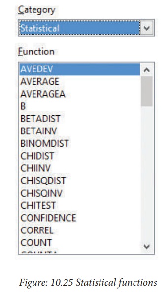
2. - Statistical functions

COUNT(Value1; Value2; ... Value30)

Counts how many numbers are in the list of arguments. Text entries are ignored. Value1; Value2; ... Value30 are 1 to 30 values or ranges representing the values to be counted.

Example

The entries 2, 4, 6 and eight in the Value 1 ... 4 fields are to be counted.

=COUNT (2;4;6;"eight") = 3. The count of numbers is therefore 3.

COUNTA(Value1; Value2; ... Value30)

Counts how many values are in the list. Text entries are also counted, even when they contain an empty string of length 0 Value1; Value2; ... Value30 are 1 to 30 arguments representing the values to be counted.

Example

The entries 2, 4, 6 and eight in the Value 1 ... 4 fields are to be counted.

=COUNTA(2;4;6;"eight") = 4. The count of values is therefore 4.

CORREL(Data1; Data2)

Returns the correlation coefficient between two data sets.Data1 is the first data set. Data2 is the second data set.

Example

=CORREL(A1:A20;B1:B20) calculates the correlation coefficient as a measure of the linear correlation of the two data sets.

LARGE(Data; Rank_C)

Returns the Rank_c-th largest value in a data set. Data is the cell range of data. Rank_C is the ranking of the value.

Example

=LARGE(A1:C50;2) gives the second largest value in the range A1:C50.

SMALL(Data; Rank_C)

Returns the Rank_c-th smallest value in a data set. Data is the cell range of data. Rank_C is the rank of the value.

Example

=SMALL(A1:C50;3) gives the third smallest value in the range A1:C50.

AVERAGE(Number1; Number2; ... Numb er20)

Returns the average of the arguments. Number1; Number2; ... Number20 are 1 to 20 numeric values or ranges.

Example

=AVERAGE(A1:A20) Returns average of set of values from the cell range A 1 : A 2 0

Working with the functions in Logical Category [w5]

IF (Test; TrueValue; FalseValue)

Specifies a logical test to be performed. Test is any value or expression that can be TRUE or FALSE. TrueValue (optional) is the value that is returned if the logical test is TRUE. FalseValue (optional) is the value that is returned if the logical test is FALSE.

Example

=IF(A1>5;”True”;"too small") If the value in A1 is higher than 5 then the text “True” is entered in the current cell otherwise the text “False” (without quotes) is entered.

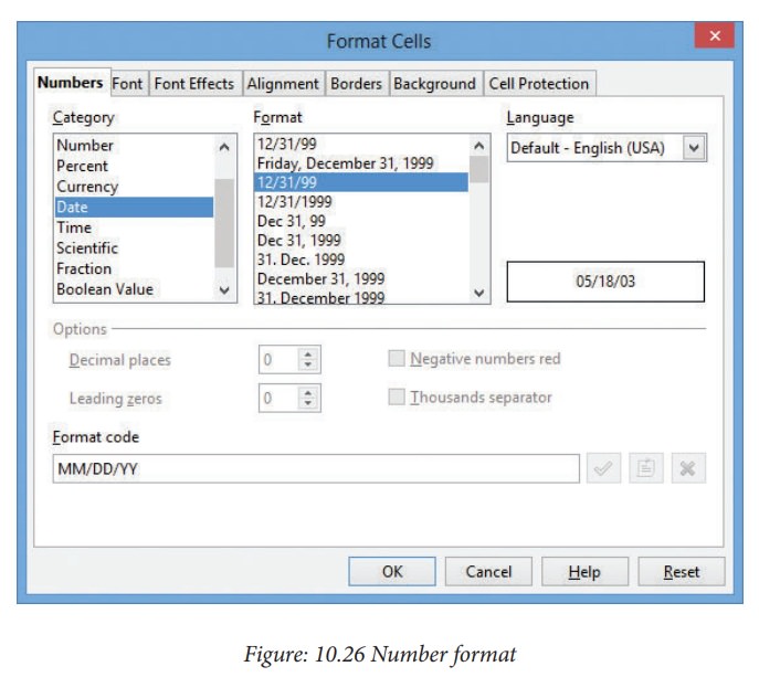
Working with the functions in Date and Time Category [w6]

OpenOffice Calc internally handles a date/time value as a numeric value. To change the number format (date or time) accordingly. To do this, select the cell containing the date or time value. Click Format menu and then Cell option in the sub-menu The Numbers tab of the Format Cells Dialog Box contains the functions for defining the number format.

Working with the functions in Text Category

CONCATENATE("Text1"; "Text2";"Text3"; ...)

Combines several text strings into one string. Text1; Text2; Text3; ... are 1 to 30 text passages which are to be concatenated together into one string.

Example

=CONCATENATE("Good  ";"Morning  ";"Mr.  ";"Ramki")  returns Good Morning Mr. Ramki

DECIMAL("Text"; Radix)

Converts a text string with characters from a number system to a positive integer in the base radix given. Text is the text string to be converted. To differentiate between a hexadecimal number, such as A1 and the reference to cell A1, you must place the number in quotation marks, for example, "A1" or "FACE". Radix indicates the base of the number system. It may be any positive integer in the range 2 to 36.

Example

=DECIMAL("17";10)        returns   17.

=DECIMAL("FACE";16)           returns     64206.

=DECIMAL("0101";2) returns 5.