Formatting Cells and Protecting Worksheets, locking and hiding cells - OpenOffice Calc

Formatting Cells and Protecting Worksheets, locking and hiding cells

Formatting Data in a cell gives additional effect to the text. Additional effect includes changing the Font type, Style, Font size, automatic wrapping, bold, underline, italic etc. The data in Calc can be formatted in several ways.

Icons available in the Formatting Tool Bar:

1.  Font Name list box:  Various fonts are available in the list from which required font can be selected.

2.  Font Size list box: Font size can be selected from this list box.

3.  Bold Icon: This icon is used to apply bold for selected cell. Key board shortcut Ctrl + B can also be used.

4.  Italic Icon: Italic icon is used to apply italic style to selected cell. Ctrl + I can also be used to apply italic.

5.  Under line Icon: To apply underline for selected cell this icon can be used. Ctrl + U can be used for this.

6.  Four alignment Icons: Using this icon content of a cell can be aligned Left, Center, Right and Justify. The key board short cuts are Ctrl + L, Ctrl + E, Ctrl + R and Ctrl + J can also be used respectively to align cell content.

7.  Number Format Icon: Currency symbol (Ctrl + Shift + 4), Percent (Ctrl + Shift + 5), Standard (Ctrl + Shift + 6), Add Decimal Place,  Delete Decimal Place can be applied using this icons.

8.  Increase Indent and Decrease Indent Icons can be used to indent the cell content.

9   Borders Icon, Background Colour Icon and Font Colour Icons can be used to apply border, to change cell background colour and to change Font colour.

Formatting using Format Cells Dialog Box:

The above formatting options can be applied individually one by one. But to apply and see preview. Format Cells dialog box is used. Select a cell and Right-click and select Format → Cells or click Edit → Cells... or press Ctrl+1, now Format Cells dialog box appears with seven tabs as follows.

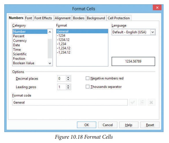
Numbers Tab :

Several number formats like Category, Format, Language, Decimal places, leading zeros and Thousands separator. User-defined Format code is also applied. Main advantage is that preview is available.

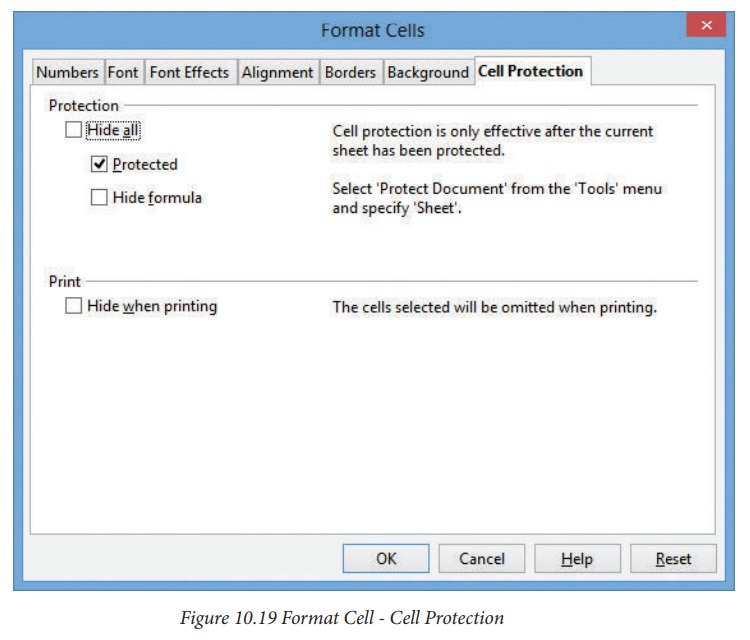
Protection Tab :

In Open Office Calc, cells are protected against any accidental changes. Protection can be provided by means of a password. Authorization is given through the correct password. It is clear that the cell protection with a Protected attribute is only effective when the whole sheet is in protected mode.

1. Select the cells that you want to specify the cell protection feature..

2. Choose Format → Cells and click the Cell Protection tab.

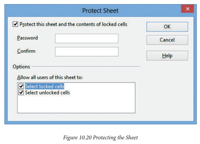
3. Select the protection options that you want. Any option can be applied only after protecting the sheet . This can be done through the menu Tools->Protect Document->Sheet. The Protected Sheet Dialog Box appears as below.

Uncheck Protected to allow the user to change the currently selected cells in the Protected Sheet Dialog box.

4. Select Protected to prevent changes to the contents and the format of a cell.

5. Select Hide formula to hide and to protect formulae from changes.

6. Select Hide when printing to hide protected cells in the printed document. (The cells are not hidden on screen).

7. Click OK.

8. Apply the protection options.

8.1 To protect the cells from being changed / viewed / printed according to your settings in the Format→ Cells Dialog box, choose Tools → Protect Document → Sheet.

8.2 Enter a password with of atleast 5 or more characters.