Design Principles of Computer Clusters

DESIGN PRINCIPLES OF COMPUTER CLUSTERS

Clusters should be designed for scalability and availability. In this section, we will cover the design principles of SSI, HA, fault tolerance, and rollback recovery in general-purpose computers and clus-ters of cooperative computers.

1. Single-System Image Features

SSI does not mean a single copy of an operating system image residing in memory, as in an SMP or a workstation. Rather, it means the illusion of a single system, single control, symmetry, and transparency as characterized in the following list:

•    Single system The entire cluster is viewed by users as one system that has multiple processors. The user could say, “Execute my application using five processors.” This is different from a distributed system.

•    Single control Logically, an end user or system user utilizes services from one place with a single interface. For instance, a user submits batch jobs to one set of queues; a system administrator configures all the hardware and software components of the cluster from one control point.

•    Symmetry A user can use a cluster service from any node. In other words, all cluster services and functionalities are symmetric to all nodes and all users, except those protected by access rights.

•    Location-transparent The user is not aware of the where abouts of the physical device that eventually provides a service. For instance, the user can use a tape drive attached to any cluster node as though it were physically attached to the local node.

The main motivation to have SSI is that it allows a cluster to be used, controlled, and main-tained as a familiar workstation is. The word “single” in “single-system image” is sometimes synon-ymous with “global” or “central.” For instance, a global file system means a single file hierarchy, which a user can access from any node. A single point of control allows an operator to monitor and configure the cluster system. Although there is an illusion of a single system, a cluster service or functionality is often realized in a distributed manner through the cooperation of multiple compo-nents. A main requirement (and advantage) of SSI techniques is that they provide both the perfor-mance benefits of distributed implementation and the usability benefits of a single image.

From the viewpoint of a process P, cluster nodes can be classified into three types. The home node of a process P is the node where P resided when it was created. The local node of a process P is the node where P currently resides. All other nodes are remote nodes to P. Cluster nodes can be configured to suit different needs. A host node serves user logins through Telnet, rlogin, or even FTP and HTTP. A compute node is one that performs computational jobs. An I/O node is one that serves file I/O requests. If a cluster has large shared disks and tape units, they are normally physi-cally attached to I/O nodes.

There is one home node for each process, which is fixed throughout the life of the process. At any time, there is only one local node, which may or may not be the host node. The local node and remote nodes of a process may change when the process migrates. A node can be configured to provide multiple functionalities. For instance, a node can be designated as a host, an I/O node, and a compute node at the same time. The illusion of an SSI can be obtained at several layers, three of which are discussed in the following list. Note that these layers may overlap with one another.

•    Application software layer Two examples are parallel web servers and various parallel databases. The user sees an SSI through the application and is not even aware that he is using a cluster. This approach demands the modification of workstation or SMP applications for clusters.

•    Hardware or kernel layer Ideally, SSI should be provided by the operating system or by the hardware. Unfortunately, this is not a reality yet. Furthermore, it is extremely difficult to provide an SSI over heterogeneous clusters. With most hardware architectures and operating systems being proprietary, only the manufacturer can use this approach.

•    Middleware layer The most viable approach is to construct an SSI layer just above the OS kernel. This approach is promising because it is platform-independent and does not require application modification. Many cluster job management systems have already adopted this approach.

Each computer in a cluster has its own operating system image. Thus, a cluster may display multiple system images due to the stand-alone operations of all participating node computers. Deter-mining how to merge the multiple system images in a cluster is as difficult as regulating many indi-vidual personalities in a community to a single personality. With different degrees of resource sharing, multiple systems could be integrated to achieve SSI at various operational levels.

1.1 Single Entry Point

Single-system image (SSI) is a very rich concept, consisting of single entry point, single file hierarchy, single I/O space, single networking scheme, single control point, single job manage-ment system, single memory space, and single process space. The single entry point enables users to log in (e.g., through Telnet, rlogin, or HTTP) to a cluster as one virtual host, although the clus-ter may have multiple physical host nodes to serve the login sessions. The system transparently distributes the user’s login and connection requests to different physical hosts to balance the load. Clusters could substitute for mainframes and supercomputers. Also, in an Internet cluster server, thousands of HTTP or FTP requests may come simultaneously. Establishing a single entry point with multiple hosts is not a trivial matter. Many issues must be resolved. The following is just a partial list:

•    Home directory Where do you put the user’s home directory?

•    Authentication How do you authenticate user logins?

•    Multiple connections What if the same user opens several sessions to the same user account?

•    Host failure How do you deal with the failure of one or more hosts?

Example 2.5 Realizing a Single Entry Point in a Cluster of Computers

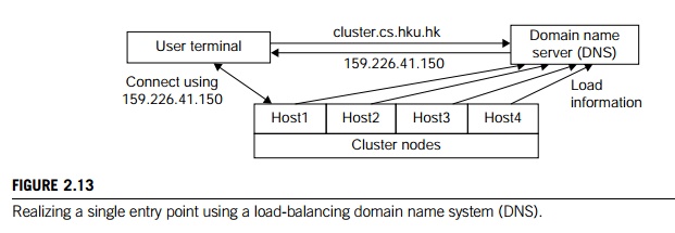
Figure 2.13 illustrates how to realize a single entry point. Four nodes of a cluster are used as host nodes to receive users’ login requests. Although only one user is shown, thousands of users can connect to the cluster in the same fashion. When a user logs into the cluster, he issues a standard UNIX command such as telnet cluster.cs.hku.hk, using the symbolic name of the cluster system.

The DNS translates the symbolic name and returns the IP address 159.226.41.150 of the least-loaded node, which happens to be node Host1. The user then logs in using this IP address. The DNS periodically receives load information from the host nodes to make load-balancing translation decisions. In the ideal case, if 200 users simultaneously log in, the login sessions are evenly distributed among our hosts with 50 users each. This allows a single host to be four times more powerful.

1.2 Single File Hierarchy

We use the term “single file hierarchy” in this book to mean the illusion of a single, huge file sys-tem image that transparently integrates local and global disks and other file devices (e.g., tapes). In other words, all files a user needs are stored in some subdirectories of the root directory /, and they can be accessed through ordinary UNIX calls such as open, read, and so on. This should not be confused with the fact that multiple file systems can exist in a workstation as subdirectories of the root directory.

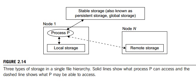
The functionalities of a single file hierarchy have already been partially provided by existing distrib-uted file systems such as Network File System (NFS) and Andrew File System (AFS). From the view-point of any process, files can reside on three types of locations in a cluster, as shown in Figure 2.14.

Local storage is the disk on the local node of a process. The disks on remote nodes are remote storage. A stable storage requires two aspects: It is persistent, which means data, once written to the stable storage, will stay there for a sufficiently long time (e.g., a week), even after the cluster shuts down; and it is fault-tolerant to some degree, by using redundancy and periodic backup to tapes.

Figure 2.14 uses stable storage. Files in stable storage are called global files, those in local sto-rage local files, and those in remote storage remote files. Stable storage could be implemented as one centralized, large RAID disk. But it could also be distributed using local disks of cluster nodes. The first approach uses a large disk, which is a single point of failure and a potential performance bottleneck. The latter approach is more difficult to implement, but it is potentially more economical, more efficient, and more available. On many cluster systems, it is customary for the system to make visible to the user processes the following directories in a single file hierarchy: the usual system directories as in a traditional UNIX workstation, such as /usr and /usr/local; and the user’s home directory ~/ that has a small disk quota (1–20 MB). The user stores his code files and other files here. But large data files must be stored elsewhere.

•    A global directory is shared by all users and all processes. This directory has a large disk space of multiple gigabytes. Users can store their large data files here.

•    On a cluster system, a process can access a special directory on the local disk. This directory has medium capacity and is faster to access than the global directory.

1.3 Visibility of Files

The term “visibility” here means a process can use traditional UNIX system or library calls such as fopen, fread, and fwrite to access files. Note that there are multiple local scratch directories in a cluster. The local scratch directories in remote nodes are not in the single file hierarchy, and are not directly visible to the process. A user process can still access them with commands such as rcp or some special library functions, by specifying both the node name and the filename.

The name “scratch” indicates that the storage is meant to act as a scratch pad for temporary information storage. Information in the local scratch space could be lost once the user logs out. Files in the global scratch space will normally persist even after the user logs out, but will be deleted by the system if not accessed in a predetermined time period. This is to free disk space for other users. The length of the period can be set by the system administrator, and usually ranges from one day to several weeks. Some systems back up the global scratch space to tapes periodically or before deleting any files.

1.4 Support of Single-File Hierarchy

It is desired that a single file hierarchy have the SSI properties discussed, which are reiterated for file systems as follows:

•    Single system There is just one file hierarchy from the user’s viewpoint.

•    Symmetry A user can access the global storage (e.g., /scratch) using a cluster service from any node. In other words, all file services and functionalities are symmetric to all nodes and all users, except those protected by access rights.

•    Location-transparent The user is not aware of the whereabouts of the physical device that eventually provides a service. For instance, the user can use a RAID attached to any cluster node as though it were physically attached to the local node. There may be some performance differences, though.

A cluster file system should maintain UNIX semantics: Every file operation (fopen, fread, fwrite, fclose, etc.) is a transaction. When an fread accesses a file after an fwrite modifies the same file, the fread should get the updated value. However, existing distributed file systems do not completely follow UNIX semantics. Some of them update a file only at close or flush. A number of alternatives have been suggested to organize the global storage in a cluster. One extreme is to use a single file server that hosts a big RAID. This solution is simple and can be easily implemented with current software (e.g., NFS). But the file server becomes both a performance bottleneck and a single point of failure. Another extreme is to utilize the local disks in all nodes to form global storage. This could solve the performance and availability problems of a single file server.

1.5 Single I/O, Networking, and Memory Space

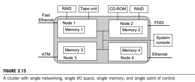
To achieve SSI, we desire a single control point, a single address space, a single job management system, a single user interface, and a single process control, as depicted in Figure 2.15. In this example, each node has exactly one network connection. Two of the four nodes each have two I/O devices attached.

Single Networking: A properly designed cluster should behave as one system (the shaded area). In other words, it is like a big workstation with four network connections and four I/O devices attached. Any process on any node can use any network and I/O device as though it were attached to the local node. Single networking means any node can access any network connection.

Single Point of Control: The system administrator should be able to configure, monitor, test, and control the entire cluster and each individual node from a single point. Many clusters help with this through a system console that is connected to all nodes of the cluster. The system console is normally connected to an external LAN (not shown in Figure 2.15) so that the administrator can log in remotely to the system console from anywhere in the LAN to perform administration work.

Note that single point of control does not mean all system administration work should be carried out solely by the system console. In reality, many administrative functions are distributed across the cluster. It means that controlling a cluster should be no more difficult than administering an SMP or a mainframe. It implies that administration-related system information (such as various configuration files) should be kept in one logical place. The administrator monitors the cluster with one graphics tool, which shows the entire picture of the cluster, and the administrator can zoom in and out at will.

Single point of control (or single point of management) is one of the most challenging issues in constructing a cluster system. Techniques from distributed and networked system management can be transferred to clusters. Several de facto standards have already been developed for network management. An example is Simple Network Management Protocol (SNMP). It demands an efficient cluster management package that integrates with the availability support system, the file system, and the job management system.

Single Memory Space: Single memory space gives users the illusion of a big, centralized main memory, which in reality may be a set of distributed local memory spaces. PVPs, SMPs, and DSMs have an edge over MPPs and clusters in this respect, because they allow a program to utilize all global or local memory space. A good way to test if a cluster has a single memory space is to run a sequential program that needs a memory space larger than any single node can provide.

Suppose each node in Figure 2.15 has 2 GB of memory available to users. An ideal single memory image would allow the cluster to execute a sequential program that needs 8 GB of memory. This would enable a cluster to operate like an SMP system. Several approaches have

been attempted to achieve a single memory space on clusters. Another approach is to let the compiler distribute the data structures of an application across multiple nodes. It is still a challenging task to develop a single memory scheme that is efficient, platform-independent, and able to support sequential binary codes.

Single I/O Address Space: Assume the cluster is used as a web server. The web information database is distributed between the two RAIDs. An HTTP daemon is started on each node to handle web requests, which come from all four network connections. A single I/O space implies that any node can access the two RAIDs. Suppose most requests come from the ATM network. It would be beneficial if the functions of the HTTP on node 3 could be distributed to all four nodes. The following example shows a distributed RAID-x architecture for I/O-centric cluster computing.

Example 2.6 Single I/O Space over Distributed RAID for I/O-Centric Clusters

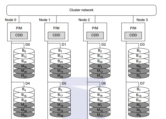
A distributed disk array architecture was proposed by Hwang, et al. [9] for establishing a single I/O space in I/O-centric cluster applications. Figure 2.16 shows the architecture for a four-node Linux PC cluster, in which three disks are attached to the SCSI bus of each host node. All 12 disks form an integrated RAID-x with a single address space. In other words, all PCs can access both local and remote disks. The addres-sing scheme for all disk blocks is interleaved horizontally. Orthogonal stripping and mirroring make it possi-ble to have a RAID-1 equivalent capability in the system.

The shaded blocks are images of the blank blocks. A disk block and its image will be mapped on dif-ferent physical disks in an orthogonal manner. For example, the block B₀ is located on disk D0. The image block M_o of block B₀ is located on disk D3. The four disks D0, D1, D2, and D3 are attached to four servers, and thus can be accessed in parallel. Any single disk failure will not lose the data block, because its image is available in recovery. All disk blocks are labeled to show image mapping. Benchmark experi-ments show that this RAID-x is scalable and can restore data after any single disk failure. The distributed RAID-x has improved aggregate I/O bandwidth in both parallel read and write operations over all physical disks in the cluster.

1.6 Other Desired SSI Features

The ultimate goal of SSI is for a cluster to be as easy to use as a desktop computer. Here are addi-tional types of SSI, which are present in SMP servers:

•    Single job management system All cluster jobs can be submitted from any node to a single job management system.

•    Single user interface The users use the cluster through a single graphical interface. Such an interface is available for workstations and PCs. A good direction to take in developing a cluster GUI is to utilize web technology.

•    Single process space All user processes created on various nodes form a single process space and share a uniform process identification scheme. A process on any node can create (e.g., through a UNIX fork) or communicate with (e.g., through signals, pipes, etc.) processes on remote nodes.

•    Middleware support for SSI clustering As shown in Figure 2.17, various SSI features are supported by middleware developed at three cluster application levels:

•    Management level This level handles user applications and provides a job management system such as GLUnix, MOSIX, Load Sharing Facility (LSF), or Codine.

•    Programming level This level provides single file hierarchy (NFS, xFS, AFS, Proxy) and distributed shared memory (TreadMark, Wind Tunnel).

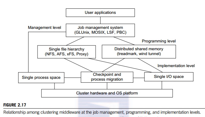
•    Implementation level This level supports a single process space, checkpointing, process migration, and a single I/O space. These features must interface with the cluster hardware and OS platform. The distributed disk array, RAID-x, in Example 2.6 implements a single I/O space.

2. High Availability through Redundancy

When designing robust, highly available systems three terms are often used together: reliability, availability, and serviceability (RAS). Availability is the most interesting measure since it combines the concepts of reliability and serviceability as defined here:

•    Reliability measures how long a system can operate without a breakdown.

•    Availability indicates the percentage of time that a system is available to the user, that is, the percentage of system uptime.

•    Serviceability refers to how easy it is to service the system, including hardware and software maintenance, repair, upgrades, and so on.

The demand for RAS is driven by practical market needs. A recent Find/SVP survey found the following figures among Fortune 1000 companies: An average computer is down nine times per year with an average downtime of four hours. The average loss of revenue per hour of downtime is $82,500. With such a hefty penalty for downtime, many companies are striving for systems that offer 24/365 availability, meaning the system is available 24 hours per day, 365 days per year.

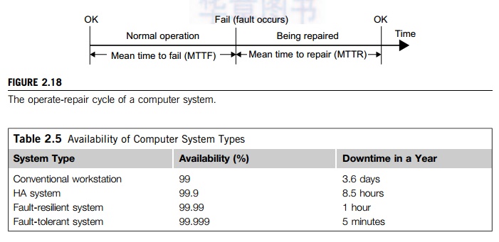
2.1 Availability and Failure Rate

As Figure 2.18 shows, a computer system operates normally for a period of time before it fails. The failed system is then repaired, and the system returns to normal operation. This operate-repair cycle then repeats. A system’s reliability is measured by the mean time to failure (MTTF), which is the average time of normal operation before the system (or a component of the system) fails. The metric for serviceability is the mean time to repair (MTTR), which is the average time it takes to repair the system and restore it to working condition after it fails. The availability of a system is defined by:

2.2 Planned versus Unplanned Failure

When studying RAS, we call any event that prevents the system from normal operation a failure. This includes:

•    Unplanned failures The system breaks, due to an operating system crash, a hardware failure, a network disconnection, human operation errors, a power outage, and so on. All these are simply called failures. The system must be repaired to correct the failure.

•    Planned shutdowns The system is not broken, but is periodically taken off normal operation for upgrades, reconfiguration, and maintenance. A system may also be shut down for weekends or holidays. The MTTR in Figure 2.18 for this type of failure is the planned downtime.

Table 2.5 shows the availability values of several representative systems. For instance, a conven-tional workstation has an availability of 99 percent, meaning it is up and running 99 percent of the time or it has a downtime of 3.6 days per year. An optimistic definition of availability does not consider planned downtime, which may be significant. For instance, many supercomputer installations have a planned downtime of several hours per week, while a telephone system cannot tolerate a downtime of a few minutes per year.

2.3 Transient versus Permanent Failures

A lot of failures are transient in that they occur temporarily and then disappear. They can be dealt with without replacing any components. A standard approach is to roll back the system to a known

state and start over. For instance, we all have rebooted our PC to take care of transient failures such as a frozen keyboard or window. Permanent failures cannot be corrected by rebooting. Some hard-ware or software component must be repaired or replaced. For instance, rebooting will not work if the system hard disk is broken.

2.4 Partial versus Total Failures

A failure that renders the entire system unusable is called a total failure. A failure that only affects part of the system is called a partial failure if the system is still usable, even at a reduced capacity. A key approach to enhancing availability is to make as many failures as possible partial failures, by systematically removing single points of failure, which are hardware or software components whose failure will bring down the entire system.

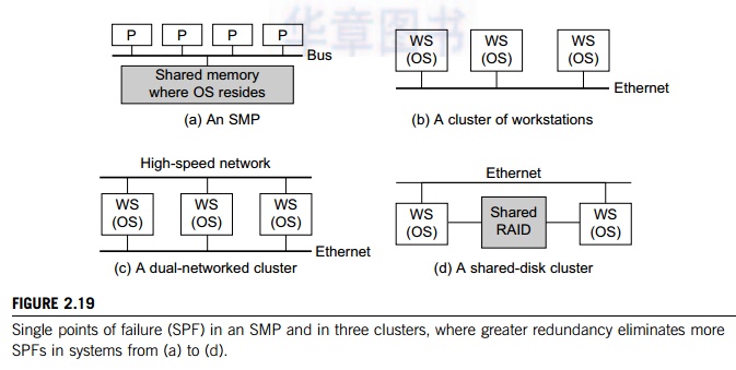
Example 2.7 Single Points of Failure in an SMP and in Clusters of Computers

In an SMP (Figure 2.19(a)), the shared memory, the OS image, and the memory bus are all single points of failure. On the other hand, the processors are not forming a single point of failure. In a cluster of work-stations (Figure 2.19(b)), interconnected by Ethernet, there are multiple OS images, each residing in a workstation. This avoids the single point of failure caused by the OS as in the SMP case. However, the Ethernet network now becomes a single point of failure, which is eliminated in Figure 2.17(c), where a high-speed network is added to provide two paths for communication.

When a node fails in the clusters in Figure 2.19(b) and Figure 2.19(c), not only will the node applications all fail, but also all node data cannot be used until the node is repaired. The shared disk cluster in Figure 2.19(d) provides a remedy. The system stores persistent data on the shared disk, and periodically checkpoints to save intermediate results. When one WS node fails, the data will not be lost in this shared-disk cluster.

2.5 Redundancy Techniques

Consider the cluster in Figure 2.19(d). Assume only the nodes can fail. The rest of the system (e.g., interconnect and the shared RAID disk) is 100 percent available. Also assume that when a node fails, its workload is switched over to the other node in zero time. We ask, what is the availability of the cluster if planned downtime is ignored? What is the availability if the cluster needs one hour/week for maintenance? What is the availability if it is shut down one hour/week, one node at a time?

According to Table 2.4, a workstation is available 99 percent of the time. The time both nodes are down is only 0.01 percent. Thus, the availability is 99.99 percent. It is now a fault-resilient sys-tem, with only one hour of downtime per year. The planned downtime is 52 hours per year, that is, 52 / (365 × 24) = 0.0059. The total downtime is now 0.59 percent + 0.01 percent = 0.6 percent. The availability of the cluster becomes 99.4 percent. Suppose we ignore the unlikely situation in which the other node fails while one node is maintained. Then the availability is 99.99 percent.

There are basically two ways to increase the availability of a system: increasing MTTF or redu-cing MTTR. Increasing MTTF amounts to increasing the reliability of the system. The computer industry has strived to make reliable systems, and today’s workstations have MTTFs in the range of hundreds to thousands of hours. However, to further improve MTTF is very difficult and costly. Clus-ters offer an HA solution based on reducing the MTTR of the system. A multinode cluster has a lower MTTF (thus lower reliability) than a workstation. However, the failures are taken care of quickly to deliver higher availability. We consider several redundancy techniques used in cluster design.

2.6 Isolated Redundancy

A key technique to improve availability in any system is to use redundant components. When a component (the primary component) fails, the service it provided is taken over by another compo-nent (the backup component). Furthermore, the primary and the backup components should be iso-lated from each other, meaning they should not be subject to the same cause of failure. Clusters provide HA with redundancy in power supplies, fans, processors, memories, disks, I/O devices, net-works, operating system images, and so on. In a carefully designed cluster, redundancy is also isolated. Isolated redundancy provides several benefits:

•    First, a component designed with isolated redundancy is not a single point of failure, and the failure of that component will not cause a total system failure.

•    Second, the failed component can be repaired while the rest of the system is still working.

•    Third, the primary and the backup components can mutually test and debug each other.

The IBM SP2 communication subsystem is a good example of isolated-redundancy design. All nodes are connected by two networks: an Ethernet network and a high-performance switch. Each node uses two separate interface cards to connect to these networks. There are two communication protocols: a standard IP and a user-space (US) protocol; each can run on either network. If either network or protocol fails, the other network or protocol can take over.

2.7 N-Version Programming to Enhance Software Reliability

A common isolated-redundancy approach to constructing a mission-critical software system is called N-version programming. The software is implemented by N isolated teams who may not even know the others exist. Different teams are asked to implement the software using different algorithms, programming languages, environment tools, and even platforms. In a fault-tolerant system, the N versions all run simultaneously and their results are constantly compared. If the results differ, the system is notified that a fault has occurred. But because of isolated redundancy, it is extremely unli-kely that the fault will cause a majority of the N versions to fail at the same time. So the system continues working, with the correct result generated by majority voting. In a highly available but less mission-critical system, only one version needs to run at a time. Each version has a built-in self-test capability. When one version fails, another version can take over.

3. Fault-Tolerant Cluster Configurations

The cluster solution was targeted to provide availability support for two server nodes with three ascending levels of availability: hot standby, active takeover, and fault-tolerant. In this section, we will consider the recovery time, failback feature, and node activeness. The level of availability increases from standby to active and fault-tolerant cluster configurations. The shorter is the recovery time, the higher is the cluster availability. Failback refers to the ability of a recovered node return-ing to normal operation after repair or maintenance. Activeness refers to whether the node is used in active work during normal operation.

•    Hot standby server clusters In a hot standby cluster, only the primary node is actively doing all the useful work normally. The standby node is powered on (hot) and running some monitoring programs to communicate heartbeat signals to check the status of the primary node, but is not actively running other useful workloads. The primary node must mirror any data to shared disk storage, which is accessible by the standby node. The standby node requires a second copy of data.

•    Active-takeover clusters In this case, the architecture is symmetric among multiple server nodes. Both servers are primary, doing useful work normally. Both failover and failback are often supported on both server nodes. When a node fails, the user applications fail over to the available node in the cluster. Depending on the time required to implement the failover, users may experience some delays or may lose some data that was not saved in the last checkpoint.

•      Failover cluster This is probably the most important feature demanded in current clusters for commercial applications. When a component fails, this technique allows the remaining system to take over the services originally provided by the failed component. A failover mechanism must provide several functions, such as failure diagnosis, failure notification, and failure recovery. Failure diagnosis refers to the detection of a failure and the location of the failed component that caused the failure. A commonly used technique is heartbeat, whereby the cluster nodes send out a stream of heartbeat messages to one another. If the system does not receive the stream of heartbeat messages from a node, it can conclude that either the node or the network connection has failed.

Example 2.8 Failure Diagnosis and Recovery in a Dual-Network Cluster

A cluster uses two networks to connect its nodes. One node is designated as the master node. Each node has a heartbeat daemon that periodically (every 10 seconds) sends a heartbeat message to the master node through both networks. The master node will detect a failure if it does not receive messages for a beat (10 seconds) from a node and will make the following diagnoses:

•    A node’s connection to one of the two networks failed if the master receives a heartbeat from the node through one network but not the other.

•    The node failed if the master does not receive a heartbeat through either network. It is assumed that the chance of both networks failing at the same time is negligible.

The failure diagnosis in this example is simple, but it has several pitfalls. What if the master node fails? Is the 10-second heartbeat period too long or too short? What if the heartbeat messages are dropped by the net-work (e.g., due to network congestion)? Can this scheme accommodate hundreds of nodes? Practical HA sys-tems must address these issues. A popular trick is to use the heartbeat messages to carry load information so that when the master receives the heartbeat from a node, it knows not only that the node is alive, but also the resource utilization status of the node. Such load information is useful for load balancing and job management.

Once a failure is diagnosed, the system notifies the components that need to know the failure event. Failure notification is needed because the master node is not the only one that needs to have this informa-tion. For instance, in case of the failure of a node, the DNS needs to be told so that it will not connect more users to that node. The resource manager needs to reassign the workload and to take over the remaining workload on that node. The system administrator needs to be alerted so that she can initiate proper actions to repair the node.

3.1 Recovery Schemes

Failure recovery refers to the actions needed to take over the workload of a failed component. There are two types of recovery techniques. In backward recovery, the processes running on a cluster per-iodically save a consistent state (called a checkpoint) to a stable storage. After a failure, the system is reconfigured to isolate the failed component, restores the previous checkpoint, and resumes nor-mal operation. This is called rollback.

Backward recovery is relatively easy to implement in an application-independent, portable fashion, and has been widely used. However, rollback implies wasted execution. If execution time is crucial, such as in real-time systems where the rollback time cannot be tolerated, a forward recovery scheme should be used. With such a scheme, the system is not rolled back to the previous checkpoint upon a failure. Instead, the system utilizes the failure diagnosis information to reconstruct a valid system state and continues execution. Forward recovery is application-dependent and may need extra hardware.

Example 2.9 MTTF, MTTR, and Failure Cost Analysis

Consider a cluster that has little availability support. Upon a node failure, the following sequence of events takes place:

1.   The entire system is shut down and powered off.

2.   The faulty node is replaced if the failure is in hardware.

3.   The system is powered on and rebooted.

4.   The user application is reloaded and rerun from the start.

Assume one of the cluster nodes fails every 100 hours. Other parts of the cluster never fail. Steps 1 through 3 take two hours. On average, the mean time for step 4 is two hours. What is the availability of the cluster? What is the yearly failure cost if each one-hour downtime costs $82,500?

Solution: The cluster’s MTTF is 100 hours; the MTTR is 2 + 2 = 4 hours. According to Table 2.5, the availability is 100/104 = 96.15 percent. This corresponds to 337 hours of downtime in a year, and the failure cost is $82500 × 337, that is, more than $27 million.

Example 2.10 Availability and Cost Analysis of a Cluster of Computers

Repeat Example 2.9, but assume that the cluster now has much increased availability support. Upon a node failure, its workload automatically fails over to other nodes. The failover time is only six minutes. Meanwhile, the cluster has hot swap capability: The faulty node is taken off the cluster, repaired, replugged, and rebooted, and it rejoins the cluster, all without impacting the rest of the cluster. What is the availability of this ideal cluster, and what is the yearly failure cost?

Solution: The cluster’s MTTF is still 100 hours, but the MTTR is reduced to 0.1 hours, as the cluster is available while the failed node is being repaired. From to Table 2.5, the availability is 100/100.5 = 99.9 percent. This corresponds to 8.75 hours of downtime per year, and the failure cost is $82,500, a 27M/722K = 38 times reduction in failure cost from the design in Example 3.8.

4. Checkpointing and Recovery Techniques

Checkpointing and recovery are two techniques that must be developed hand in hand to enhance the availability of a cluster system. We will start with the basic concept of checkpointing. This is the process of periodically saving the state of an executing program to stable storage, from which the system can recover after a failure. Each program state saved is called a checkpoint. The disk file that contains the saved state is called the checkpoint file. Although all current checkpointing soft-ware saves program states in a disk, research is underway to use node memories in place of stable storage in order to improve performance.

Checkpointing techniques are useful not only for availability, but also for program debugging, process migration, and load balancing. Many job management systems and some operating systems support checkpointing to a certain degree. The Web Resource contains pointers to numerous check-point-related web sites, including some public domain software such as Condor and Libckpt. Here we will present the important issues for the designer and the user of checkpoint software. We will first consider the issues that are common to both sequential and parallel programs, and then we will discuss the issues pertaining to parallel programs.

4.1 Kernel, Library, and Application Levels

Checkpointing can be realized by the operating system at the kernel level, where the OS transpar-ently checkpoints and restarts processes. This is ideal for users. However, checkpointing is not sup-ported in most operating systems, especially for parallel programs. A less transparent approach links the user code with a checkpointing library in the user space. Checkpointing and restarting are handled by this runtime support. This approach is used widely because it has the advantage that user applications do not have to be modified.

A main problem is that most current checkpointing libraries are static, meaning the application source code (or at least the object code) must be available. It does not work if the application is in the form of executable code. A third approach requires the user (or the compiler) to insert check-pointing functions in the application; thus, the application has to be modified, and the transparency is lost. However, it has the advantage that the user can specify where to checkpoint. This is helpful to reduce checkpointing overhead. Checkpointing incurs both time and storage overheads.

4.2 Checkpoint Overheads

During a program’s execution, its states may be saved many times. This is denoted by the time consumed to save one checkpoint. The storage overhead is the extra memory and disk space required for checkpointing. Both time and storage overheads depend on the size of the checkpoint file. The overheads can be substantial, especially for applications that require a large memory space. A number of techniques have been suggested to reduce these overheads.

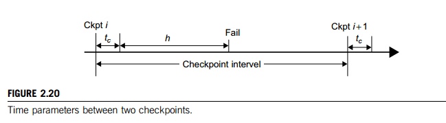
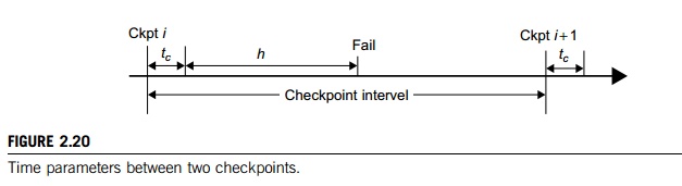
4.3 Choosing an Optimal Checkpoint Interval

The time period between two checkpoints is called the checkpoint interval. Making the interval larger can reduce checkpoint time overhead. However, this implies a longer computation time after a failure. Wong and Franklin [28] derived an expression for optimal checkpoint interval as illu-strated in Figure 2.20.

Here, MTTF is the system’s mean time to failure. This MTTF accounts the time consumed to save one checkpoint, and h is the average percentage of normal computation performed in a check-point interval before the system fails. The parameter h is always in the range. After a system is restored, it needs to spend h × (checkpoint interval) time to recompute.

4.4 Incremental Checkpoint

Instead of saving the full state at each checkpoint, an incremental checkpoint scheme saves only the portion of the state that is changed from the previous checkpoint. However, care must be taken regarding old checkpoint files. In full-state checkpointing, only one checkpoint file needs to be kept on disk. Subsequent checkpoints simply overwrite this file. With incremental checkpointing, old files needed to be kept, because a state may span many files. Thus, the total storage requirement is larger.

4.5 Forked Checkpointing

Most checkpoint schemes are blocking in that the normal computation is stopped while checkpoint-ing is in progress. With enough memory, checkpoint overhead can be reduced by making a copy of the program state in memory and invoking another asynchronous thread to perform the checkpointing concurrently. A simple way to overlap checkpointing with computation is to use the UNIX fork( ) system call. The forked child process duplicates the parent process’s address space and checkpoints it. Meanwhile, the parent process continues execution. Overlapping is achieved since checkpointing is disk-I/O intensive. A further optimization is to use the copy-on-write mechanism.

4.6 User-Directed Checkpointing

The checkpoint overheads can sometimes be substantially reduced if the user inserts code (e.g., library or system calls) to tell the system when to save, what to save, and what not to save. What should be the exact contents of a checkpoint? It should contain just enough information to allow a system to recover. The state of a process includes its data state and control state. For a UNIX process, these states are stored in its address space, including the text (code), the data, the stack segments, and the process descriptor. Saving and restoring the full state is expensive and sometimes impossible.

For instance, the process ID and the parent process ID are not restorable, nor do they need to be saved in many applications. Most checkpointing systems save a partial state. For instance, the code seg-ment is usually not saved, as it does not change in most applications. What kinds of applications can be checkpointed? Current checkpoint schemes require programs to be well behaved, the exact meaning of which differs in different schemes. At a minimum, a well-behaved program should not need the exact contents of state information that is not restorable, such as the numeric value of a process ID.

4.7 Checkpointing Parallel Programs

We now turn to checkpointing parallel programs. The state of a parallel program is usually much larger than that of a sequential program, as it consists of the set of the states of individual processes, plus the state of the communication network. Parallelism also introduces various timing and consistency problems.

Example 2.11 Checkpointing a Parallel Program

Figure 2.21 illustrates checkpointing of a three-process parallel program. The arrows labeled x, y, and z represent point-to-point communication among the processes. The three thick lines labeled a, b, and c represent three global snapshots (or simply snapshots), where a global snapshot is a set of checkpoints

(represented by dots), one from every process. In addition, some communication states may need to be saved. The intersection of a snapshot line with a process’s time line indicates where the process should take a (local) checkpoint. Thus, the program’s snapshot c consists of three local checkpoints: s, t, u for processes P, Q, and R, respectively, plus saving the communication y.

4.8 Consistent Snapshot

A global snapshot is called consistent if there is no message that is received by the checkpoint of one process, but not yet sent by another process. Graphically, this corresponds to the case that no arrow crosses a snapshot line from right to left. Thus, snapshot a is consistent, because arrow x is from left to right. But snapshot c is inconsistent, as y goes from right to left. To be consistent, there should not be any zigzag path between two checkpoints [20]. For instance, checkpoints u and s can-not belong to a consistent global snapshot. A stronger consistency requires that no arrows cross the snapshot. Thus, only snapshot b is consistent in Figure 2.23.

4.9 Coordinated versus Independent Checkpointing

Checkpointing schemes for parallel programs can be classified into two types. In coordinated check-pointing (also called consistent checkpointing), the parallel program is frozen, and all processes are checkpointed at the same time. In independent checkpointing, the processes are checkpointed inde-pendent of one another. These two types can be combined in various ways. Coordinated check-pointing is difficult to implement and tends to incur a large overhead. Independent checkpointing has a small overhead and can utilize existing checkpointing schemes for sequential programs.