Working With Data: Inferential Statistics

Inferential Statistics

The statistics we’ve considered so far allow us to summarize the data we’ve collected, but we often want to do more than this. We want to reach beyond our data and make broader claims—usually claims about the correctness (or the falsity) of our hypothesis. For this purpose, we need to make inferences based on our data—and so we turn to inferential statistics.

TESTING DIFFERENCES

In the example we’ve been discussing, we began with a question: Do boys and girls dif-fer in how aggressive they are? This comparison is easy for our sample because we know that in the (fictional) data we’ve collected, the boys’ mean level of aggression is 17, and the girls’ mean is 12. Obviously, the boys’ scores are higher—providing a clear answer to our question for this sample. Ultimately, though, the sample isn’t our concern. Instead,we want to make claims about a broader population; and so we still want to ask: Are boys in general (i.e., boys outside of our sample) more aggressive than girls in general?

To answer this question, we need to make some estimates based on our sample. Researchers use specific calculations for this purpose, but leaving the details aside, these calculations center on three points. First, how big a difference is found in the sample? In our example, the effect size—the difference between the groups—is 5 units (this is the difference between the boys’ average, 17, and the girls’ average, 12). In gen-eral, the larger the effect size, the more likely it is that the result can be taken at face value.

Second, how great is the variability of the data? The logic here is straightforward: If the variability in our sample is low, essentially this means that we kept seeing the same scores again and again. In that case, we’re likely to continue getting the same scores if we look beyond our sample—and so we should be more comfortable in extrapolating from our sample. If, on the other hand, the data in our sample are highly variable, then we know that the broader population is diverse—so if we looked beyond this sample, we might find much higher scores or much lower ones. In this case, we’d have to be much more cautious in drawing conclusions from our sample.

Third, how many observations does the data set include? All things being equal, the greater the number of observations, the more likely the sample is to reflect the proper-ties of the broader population. Thus, the greater the number of observations, the more trust we can put in our results.

Let’s be clear, though, that these three factors—effect size, variability, and number of observations—can trade off against each other. If, for example, the effect size is small, then we will draw conclusions from our data only if we’re certain that our measure-ments are quite accurate—and so we will insist on a low level of variability and a large number of observations. Similarly, if the variability is very low, then there’s no reason to collect a huge amount of data—this would simply give us the same observations, over and over. Therefore, with low variability, we need relatively few data points.

These trade-offs are, in fact, built directly into the calculations researchers use to evaluate the statistical significance of a result. This calculation takes as its input the effect size, the variability, and the number of observations; and ultimately, its output is something called a p-value. This value is literally the probability of getting the data pat-tern we did purely by accident. After all, we know that peculiar accidents can happen: Sometimes, when you toss a coin, you get five “heads” in a row, entirely by chance. When you’re rolling dice, you might—just by luck—go 30 or 40 rolls without rolling a seven. Our calculations tell us whether the result in our experiment is a similar sort of fluke—a chance occurrence only.

What could “chance” mean in the context of our comparison between boys and girls? Bear in mind that some boys are simply more aggressive than others, and likewise for girls. So it’s possible that—just by luck—our sample of boys happens to include a couple of particularly aggressive individuals who are driving up the group’s average. It’s also possible that—again, just by luck—our sample of girls includes several especially well-behaved individuals who are driving the group’s average down. This is the sort of possibility that our statistics evaluate—by asking how consistent the results are (meas-ured by the variability) as well as how likely it is that just a few chance observations (e.g., a few misbehaved boys or a few especially docile girls) could be causing the differ-ence we’ve observed between the groups (i.e., the effect size).

If the p-value we calculate is high, then we’ve observed an outcome that could easily occur by chance. In that case, we would cautiously conclude that our result might have been a random fluke, and so we should draw no conclusions from our data. If the p-value is low (i.e., we observe an outcome that would rarely occur by chance), we conclude the opposite—the outcome is likely not the product of chance and should be taken seriously.

In most cases, psychologists use a 5% rule for making this determination— usually expressed with the cutoff of p < .05. In other words, if the probability of getting a particular outcome just by chance is less than 5%, then we conclude that the particular result we observed is unlikely to be an accident. Let’s note, though, that there’s nothing sacred about this 5% rule. We use other, stricter rules when evaluat-ing especially important results or when considering patterns of evidence rather than just a single result.

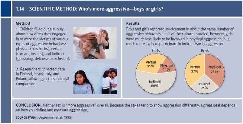
So, with all of this said, what’s the actual difference between boy’s and girl’s aggression—with real data, not the fictional data we’ve been considering so far (Figure 1.14)? The answer, with carefully collected data, turns out to depend on how exactly we define the dependent variable. If we measure physical aggression—pushing, physical intimidation, punching, kicking, biting—then males do tend to be more aggressive; and it doesn’t matter whether we’re considering children or adults, or whether we assess males in Western cultures or Eastern (e.g., Geary & Bjorklund, 2000). On the other hand, if we measure social aggression—ignoring someone, gossiping about someone, trying to isolate someone from their friends—then the evi-dence suggests that females are, in this regard, the more aggressive sex (Oesterman et al., 1998). Clearly, our answer is complicated—and this certainly turns out to be a study in which defining the dependent variable is crucial.