Working With Data: Descriptive Statistics

Descriptive Statistics

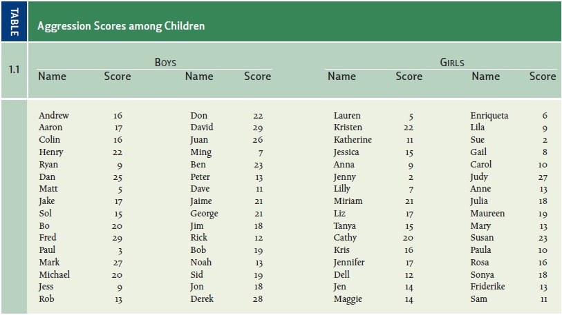
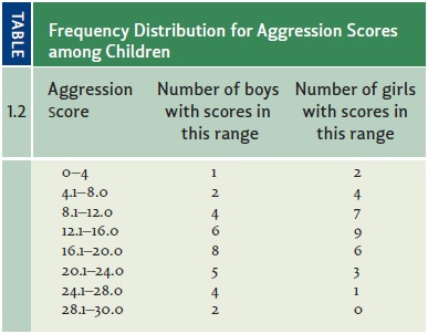
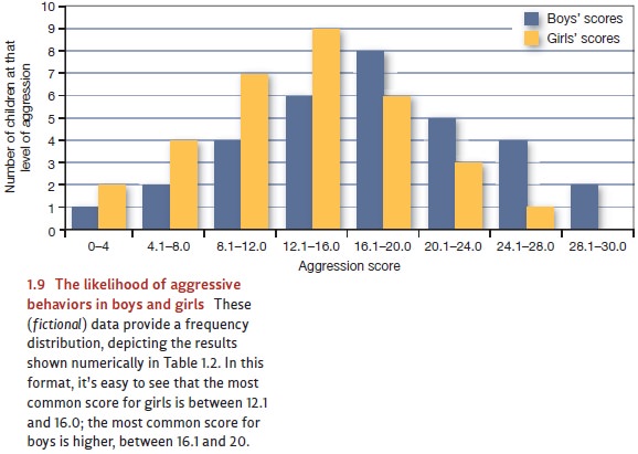
In Table 1.1, it’s difficult to see any pattern at all. Some of the boys’ numbers are high, and some are lower; the same is true for the girls. With the data in this format, it’s hard to see anything beyond these general points. The pattern becomes obvious, however, if we summarize these data in terms of a frequency distribution (Table 1.2)—a table that lists how many scores fall into each of the designated categories. The pattern is clearer still if we graph the frequency distributions (Figure 1.9). Now we  most common scores (in these fictional data) are between 16.1 and 20 for the boys andbetween 12.1 and 16.0 for the girls. As we move further and furtherfrom  these  central  categories  (looking  either  at  higher  scores  orlower), the number of people at each level of aggression drops.

MEANS AND VARIABILITY

The distribution of scores in Table 1.1 yields a graph in Figure 1.9 that is roughly bell shaped. In fact, this shape is extremely common when we graph frequency distributions—whether the graph shows the frequency of various heights among 8-year-olds, or the frequency of going to the movies among college students, or the frequency of particular test scores for a college exam. In each of these cases, there tends to be a large number of moderate values and then fewer and fewer values as we move away from the center.

To describe these curves, it’s usually enough to specify just two attributes. First, we must locate the curve’s center. This gives us a measure of the “average case” within the data set—technically,

we’re looking for a measure of central tendency of these data. The most common way of determining this average is to add up all the scores and then divide that sum by the number of scores in the set; this process yields the mean. But there are other ways of defining the average. For example, sometimes it’s convenient to refer to the median, which is the score that separates the top 50% of the scores from the bottom 50%.

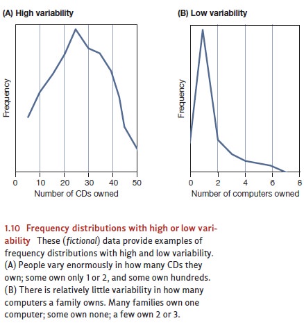
The second characteristic of a frequency distribution is its variability, which is a measure of how much the individual scores differ from one to the next. A highly vari-able data set includes a wide range of values and yields a broad, relatively flat frequency distribution like the one in Figure 1.10A. In contrast, a data set with low variability has values more tightly clustered together and yields a narrow, rather steep frequency distri-bution like the one in Figure 1.10B.

We can measure the variability in a data set in several ways, but the most common is the standard deviation. To compute the standard deviation, we first locate the center of the data set—the mean. Next, for each data point, we ask: How far away is this point from the mean? We compute this distance by simply subtracting the value for that point from the mean, and the result is the deviation for that point—that is, how much the point “deviates” from the average case. We then pool the deviations for all the points in our data set, so that we know overall how much the data deviate from the mean. If the points tend to deviate from the mean by a lot, the standard deviation will have a large value— telling us that the data set is highly variable. If the points all tend to be close to the mean, the standard deviation will be small—and thus the variability is low.

CORRELATIONS

In  describing  the  data  they  collect, investigators  also  find  it  useful  in  many  cases  to draw on another statistical measure: one that examines correlations.

Returning to our example, imagine that a researcher examines the data shown in Table 1.1 and wonders why some boys are more aggressive than others, and likewise for girls. Could it just be their age—so that, perhaps, the older children are better at con- trolling themselves? To explore this possibility, the researcher might create a scatter plot ike the one shown in Figure 1.11. In this plot, each point represents one child; the child’s age determines the horizontal position of the point within the graph, and his or her aggression score determines the vertical position.

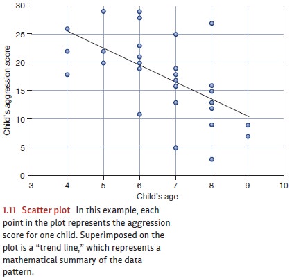
The  pattern  in  this  scatter  plot  suggests  that  these  two measurements—age  and  aggression  score—are  linked, but in  a  negative  direction. Older  children  (points  to  the  right on  the  scatter  plot)  tend  to  have  lower  aggression  scores (points lower down in the diagram). This relationship isn’t perfect; if  it  were, all  the  points  would  fall  on  the  diagonal line shown in the figure. Still, the overall pattern of the scat- ter plot indicates a relationship: If we know a child’s age, we can make a reasonable prediction about her aggression level, and vice versa.

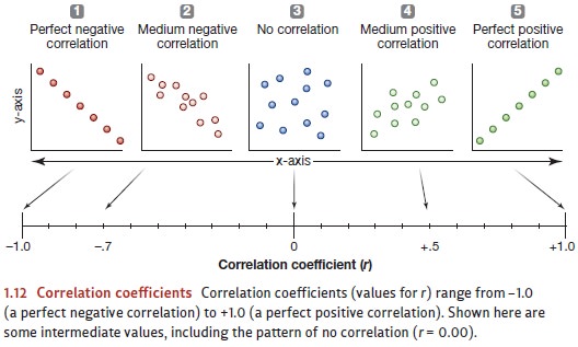
To assess data like these, researchers usually rely on a meas- ure called the correlation coefficient, symbolized by the letter r. This coefficient is always calculated on pairs of observations. In our example, the pairs consist of each child’s age and his or her aggression score; but, of  course, other  correlations involve  other pairings. Correlation  coefficients can take any value between +1.00 and –1.00 (Figure 1.12). In either of these extreme cases, the correlation  is  perfect.  For  the  data  shown  in  Figure  1.11,  a  calculation  shows  that r  = –.60. This is a reasonably strong negative correlation, but it’s obviously different from  –1.00,  thus  confirming  what  we  already  know—namely,  that  the  correlation between age and aggression score is not perfect.

Many of the relationships psychologists study yield r values in the ballpark of .40 to .60. These numbers reflect relationships strong enough to produce an easily visible pat-tern in the data. But, at the same time, these numbers indicate relationships that are far from perfect—so they certainly allow room for exceptions. To use a concrete example, consider the correlation between an individual’s height and his or her sex. When exam-ined statistically, this relationship yields a value of r = +.43. The correlation is strong enough that we can easily observe the pattern in everyday experience: With no coach-ing and no calculations, people easily detect that men, overall, tend to be taller than women. But, at the same time, we can easily think of exceptions to the overall pattern— women who are tall or men who are short. This is the sort of correlation psychologists work with all the time—strong enough to be informative, yet still allowing relatively common exceptions.

Let’s be clear, though, that the strength of a correlation—and therefore the consis-tency of the relationship revealed by the correlation—is independent of the sign of the r value. A correlation of +.43 is no stronger than a correlation of –.43, and correlationsof –1.00 and +1.00 both reflect perfectly consistent relationships.

CORRELATION SANDRELIABILITY

In any science, researchers need to have faith in their measurements: A physicist needs to be confident that her accelerometer is properly calibrated; a chemist needs a reliable spectrometer. Concerns about measurements are particularly salient in psychology, though, because we often want to assess things that resist being precisely defined— things like personality traits or mental abilities. So, how can we make sure our measurements are trustworthy? The answer often involves correlations—and this is one of several reasons that correlations are such an important research tool.

Imagine that you step onto your bathroom scale, and it shows that you’ve lost 3 pounds since last week. On reflection, you might be puzzled by this; what about that huge piece of pie you ate yesterday? For caution’s sake, you step back onto the scale and now it gives you a different reading: You haven’t lost 3 pounds at all; you’ve gained a pound. At that point, you’d probably realize you can’t trust your scale; you need one that’s more reliable.

This example suggests one way we can evaluate a measure: by examining its reliability—an assessment of howconsistentthe measure is in its results, and one pro-cedure for assessing reliability follows exactly the sequence you used with the bathroom scale: You took the measure once, let some time pass, and then took the same measure again. If the measure is reliable, then we should find a correlation between these obser-vations. Specifically, this correlation will give us an assessment of the measure’s test-retest reliability.

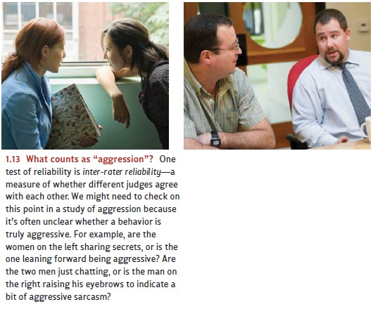
A different aspect of reliability came up in our earlier discussion: In measuring aggres-sion, we might worry that a gesture or a remark that seems aggressive to one observer may not seem that way to someone else (Figure 1.13). We thus need to guard against the possibility that our data are idiosyncratic—merely reflecting what one person regards as aggressive. To deal with this concern, we suggested that we might have a panel of judges observe the behaviors in question and that we’d trust the data only if the judges agree with each other reasonably well. This procedure relies on a different type of reliability, called inter-rater reliability, that’s calculated roughly as the correlation between Judge 1’s ratings and Judge 2’s ratings, between Judge 2’s ratings and Judge 3’s, and so on.

VALIDITY OF AMEASURE

Imagine that no matter who steps on your bathroom scale, it always shows a weight of 137 pounds. This scale would be quite reliable—but it would also be worthless, and so clearly we need more than reliability. We also need our dependent variable to measure what we intend it to measure. Likewise, if our panel of judges agrees, perhaps they’re all being misled in the same way. Maybe the judges are really focusing on how cute the var-ious boys and girls in the study are, so they’re heavily biased by the cuteness when they judge aggression. In this case, too, the judges might agree with each other—and so they’d be reliable—but the aggression scores would still be inaccurate.

These points illustrate the importance of validity—the assessment of whether the variable measures what it’s supposed to measure. There are many ways to assess valid-ity, and correlations play a central role here too. For example, intelligence is often meas-ured via some version of the IQ test, but are these tests valid? If they are, then this would mean that people with high IQ’s are actually smarter—so they should do better in activities that require smartness. We can test this proposal by asking whether IQ scores are correlated with school performance, or with measures of performance in the workplace (particularly for jobs involving some degree of complexity). It turns out that these various measures are positively correlated, thus providing a strong suggestion that IQ tests are measuring what we intend them to.