Variable Size Decrease Algorithms

Variable-Size-Decrease Algorithms

1. Computing a Median and the Selection Problem

2. Interpolation Search

3. Searching and Insertion in a Binary Search Tree

4. The Game of Nim

5. Exercises

In the third principal variety of decrease-and-conquer, the size reduction pattern varies from one iteration of the algorithm to another. Euclid’s algorithm for computing the greatest common divisor (Section 1.1) provides a good example of this kind of algorithm. In this section, we encounter a few more examples of this variety.

Computing a Median and the Selection Problem

The selection problem is the problem of finding the kth smallest element in a list of n numbers. This number is called the kth order statistic. Of course, for k = 1 or k = n, we can simply scan the list in question to find the smallest or largest element, respectively. A more interesting case of this problem is for k = n/2 , which asks to find an element that is not larger than one half of the list’s elements and not smaller than the other half. This middle value is called the median, and it is one of the most important notions in mathematical statistics. Obviously, we can find the kth smallest element in a list by sorting the list first and then selecting the kth element in the output of a sorting algorithm. The time of such an algorithm is determined by the efficiency of the sorting algorithm used. Thus, with a fast sorting algorithm such as mergesort (discussed in the next chapter), the algorithm’s efficiency is in

O(n log n).

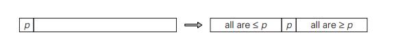
You should immediately suspect, however, that sorting the entire list is most likely overkill since the problem asks not to order the entire list but just to find its kth smallest element. Indeed, we can take advantage of the idea of partitioning a given list around some value p of, say, its first element. In general, this is a rearrangement of the list’s elements so that the left part contains all the elements smaller than or equal to p, followed by the pivot p itself, followed by all the elements greater than or equal to p.

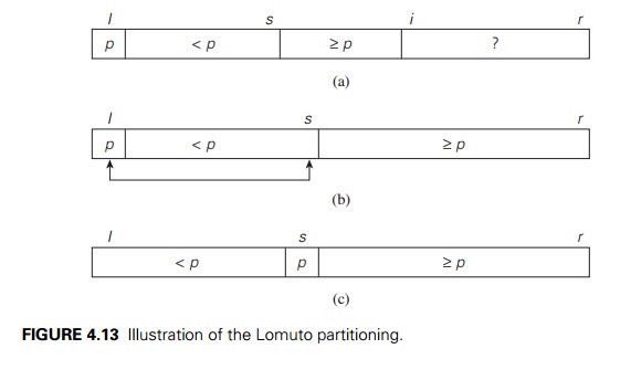
Of the two principal algorithmic alternatives to partition an array, here we discuss the Lomuto partitioning [Ben00, p. 117]; we introduce the better known Hoare’s algorithm in the next chapter. To get the idea behind the Lomuto parti-tioning, it is helpful to think of an array—or, more generally, a subarray A[l..r] (0 ≤ l ≤ r ≤ n − 1)—under consideration as composed of three contiguous seg-ments. Listed in the order they follow pivot p, they are as follows: a segment with elements known to be smaller than p, the segment of elements known to be greater than or equal to p, and the segment of elements yet to be compared to p (see Fig-ure 4.13a). Note that the segments can be empty; for example, it is always the case for the first two segments before the algorithm starts.

Starting with i = l + 1, the algorithm scans the subarray A[l..r] left to right, maintaining this structure until a partition is achieved. On each iteration, it com-pares the first element in the unknown segment (pointed to by the scanning index i in Figure 4.13a) with the pivot p. If A[i] ≥ p, i is simply incremented to expand the segment of the elements greater than or equal to p while shrinking the un-processed segment. If A[i] < p, it is the segment of the elements smaller than p that needs to be expanded. This is done by incrementing s, the index of the last element in the first segment, swapping A[i] and A[s], and then incrementing i to point to the new first element of the shrunk unprocessed segment. After no un-processed elements remain (Figure 4.13b), the algorithm swaps the pivot with A[s] to achieve a partition being sought (Figure 4.13c).

Here is pseudocode implementing this partitioning procedure.

ALGORITHM     LomutoPartition(A[l..r])

//Partitions subarray by Lomuto’s algorithm using first element as pivot //Input: A subarray A[l..r] of array A[0..n − 1], defined by its left and right

            indices l and r (l ≤ r)

//Output: Partition of A[l..r] and the new position of the pivot p ← A[l]

s ← l

for i ← l + 1 to r do

if A[i] < p

s ← s + 1; swap(A[s], A[i]) swap(A[l], A[s])

return s

How can we take advantage of a list partition to find the kth smallest element in it? Let us assume that the list is implemented as an array whose elements are indexed starting with a 0, and let s be the partition’s split position, i.e., the index of the array’s element occupied by the pivot after partitioning. If s = k − 1, pivot p itself is obviously the kth smallest element, which solves the problem. If s > k − 1, the kth smallest element in the entire array can be found as the kth smallest element in the left part of the partitioned array. And if s < k − 1, it can be found as the (k − s)th smallest element in its right part. Thus, if we do not solve the problem outright, we reduce its instance to a smaller one, which can be solved by the same approach, i.e., recursively. This algorithm is called quickselect.

To find the kth smallest element in array A[0..n − 1] by this algorithm, call

Quickselect(A[0..n − 1], k) where

ALGORITHM                 Quickselect(A[l..r], k)

//Solves the selection problem by recursive partition-based algorithm //Input: Subarray A[l..r] of array A[0..n − 1] of orderable elements and

            integer k (1 ≤ k ≤ r − l + 1)

//Output: The value of the kth smallest element in A[l..r]

s ← LomutoPartition(A[l..r]) //or another partition algorithm if s = k − 1 return A[s]

else if s > l + k − 1 Quickselect(A[l..s − 1], k) else Quickselect(A[s + 1..r], k − 1 − s)

In fact, the same idea can be implemented without recursion as well. For the nonrecursive version, we need not even adjust the value of k but just continue until s = k − 1.

EXAMPLE Apply the partition-based algorithm to find the median of the fol-lowing list of nine numbers: 4, 1, 10, 8, 7, 12, 9, 2, 15. Here, k = 9/2 = 5 and our task is to find the 5th smallest element in the array.

We use the above version of array partitioning, showing the pivots in bold.

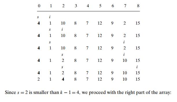
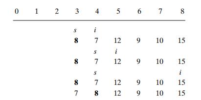
Now s = k − 1 = 4, and hence we can stop: the found median is 8, which is greater than 2, 1, 4, and 7 but smaller than 12, 9, 10, and 15.

How efficient is quickselect? Partitioning an n-element array always requires n − 1 key comparisons. If it produces the split that solves the selection problem

without requiring more iterations, then for this best case we obtain C_best (n) = n − 1 ∈  (n). Unfortunately, the algorithm can produce an extremely unbalanced

partition of a given array, with one part being empty and the other containing n − 1 elements. In the worst case, this can happen on each of the n − 1 iterations. (For a specific example of the worst-case input, consider, say, the case of k = n and a strictly increasing array.) This implies that

C_worst (n) = (n − 1) + (n − 2) + ^{. . .} + 1 = (n − 1)n/2 ∈  (n²),

which compares poorly with the straightforward sorting-based approach men-tioned in the beginning of our selection problem discussion. Thus, the usefulness of the partition-based algorithm depends on the algorithm’s efficiency in the average case. Fortunately, a careful mathematical analysis has shown that the average-case efficiency is linear. In fact, computer scientists have discovered a more sophisti-cated way of choosing a pivot in quickselect that guarantees linear time even in the worst case [Blo73], but it is too complicated to be recommended for practical applications.

It is also worth noting that the partition-based algorithm solves a somewhat more general problem of identifying the k smallest and n − k largest elements of a given list, not just the value of its kth smallest element.

Interpolation Search

As the next example of a variable-size-decrease algorithm, we consider an algo-rithm for searching in a sorted array called interpolation search. Unlike binary search, which always compares a search key with the middle value of a given sorted array (and hence reduces the problem’s instance size by half), interpolation search takes into account the value of the search key in order to find the array’s element to be compared with the search key. In a sense, the algorithm mimics the way we

search for a name in a telephone book: if we are searching for someone named Brown, we open the book not in the middle but very close to the beginning, unlike our action when searching for someone named, say, Smith.

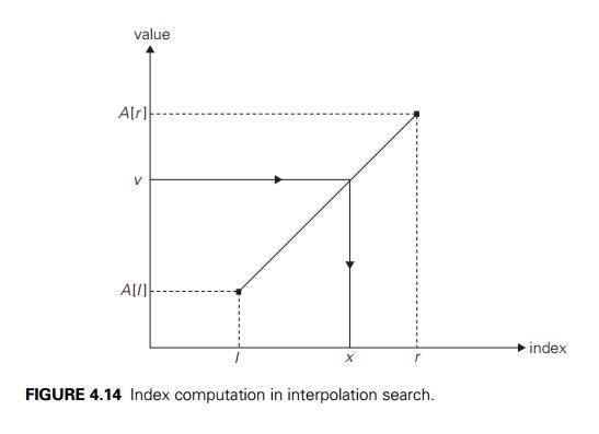
More precisely, on the iteration dealing with the array’s portion between the leftmost element A[l] and the rightmost element A[r], the algorithm assumes that the array values increase linearly, i.e., along the straight line through the points (l, A[l]) and (r, A[r]). (The accuracy of this assumption can influence the algorithm’s efficiency but not its correctness.) Accordingly, the search key’s value v is compared with the element whose index is computed as (the round-off of) the x coordinate of the point on the straight line through the points (l, A[l]) and (r, A[r]) whose y coordinate is equal to the search value v (Figure 4.14).

Writing down a standard equation for the straight line passing through the points (l, A[l]) and (r, A[r]), substituting v for y, and solving it for x leads to the following formula:

The logic behind this approach is quite straightforward. We know that the array values are increasing (more accurately, not decreasing) from A[l] to A[r], but we do not know how they do it. Had these values increased linearly, which is the simplest manner possible, the index computed by formula (4.4) would be the expected location of the array’s element with the value equal to v. Of course, if v is not between A[l] and A[r], formula (4.4) need not be applied (why?).

After comparing v with A[x], the algorithm either stops (if they are equal) or proceeds by searching in the same manner among the elements indexed either between l and x − 1 or between x + 1 and r, depending on whether A[x] is smaller or larger than v. Thus, the size of the problem’s instance is reduced, but we cannot tell a priori by how much.

The analysis of the algorithm’s efficiency shows that interpolation search uses fewer than log₂ log₂ n + 1 key comparisons on the average when searching in a list of n random keys. This function grows so slowly that the number of comparisons is a very small constant for all practically feasible inputs (see Problem 6 in this section’s exercises). But in the worst case, interpolation search is only linear, which must be considered a bad performance (why?).

Assessing the worthiness of interpolation search versus that of binary search, Robert Sedgewick wrote in the second edition of his Algorithms that binary search is probably better for smaller files but interpolation search is worth considering for large files and for applications where comparisons are particularly expensive or access costs are very high. Note that in Section 12.4 we discuss a continuous counterpart of interpolation search, which can be seen as one more example of a variable-size-decrease algorithm.

Searching and Insertion in a Binary Search Tree

Let us revisit the binary search tree. Recall that this is a binary tree whose nodes contain elements of a set of orderable items, one element per node, so that for every node all elements in the left subtree are smaller and all the elements in the right subtree are greater than the element in the subtree’s root. When we need to search for an element of a given value v in such a tree, we do it recursively in the following manner. If the tree is empty, the search ends in failure. If the tree is not empty, we compare v with the tree’s root K(r). If they match, a desired element is found and the search can be stopped; if they do not match, we continue with the search in the left subtree of the root if v < K(r) and in the right subtree if v > K(r). Thus, on each iteration of the algorithm, the problem of searching in a binary search tree is reduced to searching in a smaller binary search tree. The most sensible measure of the size of a search tree is its height; obviously, the decrease in a tree’s height normally changes from one iteration to another of the binary tree search—thus giving us an excellent example of a variable-size-decrease algorithm.

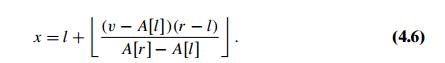
In the worst case of the binary tree search, the tree is severely skewed. This happens, in particular, if a tree is constructed by successive insertions of an increasing or decreasing sequence of keys (Figure 4.15).

Obviously, the search for a_n−1 in such a tree requires n comparisons, making the worst-case efficiency of the search operation fall into  (n). Fortunately, the average-case efficiency turns out to be in  (log n). More precisely, the number of key comparisons needed for a search in a binary search tree built from n random keys is about 2ln n ≈ 1.39 log₂ n. Since insertion of a new key into a binary search tree is almost identical to that of searching there, it also exemplifies the variable-size-decrease technique and has the same efficiency characteristics as the search operation.

The Game of Nim

There are several well-known games that share the following features. There are two players, who move in turn. No randomness or hidden information is permitted: all players know all information about gameplay. A game is impartial: each player has the same moves available from the same game position. Each of a finite number of available moves leads to a smaller instance of the same game. The game ends with a win by one of the players (there are no ties). The winner is the last player who is able to move.

A prototypical example of such games is Nim. Generally, the game is played with several piles of chips, but we consider the one-pile version first. Thus, there is a single pile of n chips. Two players take turns by removing from the pile at least one and at most m chips; the number of chips taken may vary from one move to another, but both the lower and upper limits stay the same. Who wins the game by taking the last chip, the player moving first or second, if both players make the best moves possible?

Let us call an instance of the game a winning position for the player to move next if that player has a winning strategy, i.e., a sequence of moves that results in a victory no matter what moves the opponent makes. Let us call an instance of the game a losing position for the player to move next if every move available for that player leads to a winning position for the opponent. The standard approach to determining which positions are winning and which are losing is to investigate small values of n first. 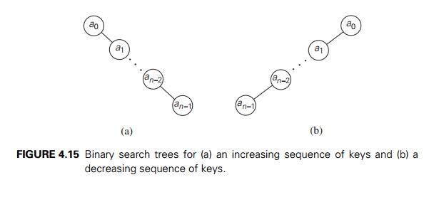It is logical to consider the instance of n = 0 as a losing one for the player to move next because this player is the first one who cannot make a move. Any instance with 1 ≤ n ≤ m chips is obviously a winning position for the player to move next (why?). The instance with n = m + 1 chips is a losing one because taking any allowed number of chips puts the opponent in a winning position. (See an illustration for m = 4 in Figure 4.16.) Any instance with m + 2 ≤ n ≤ 2m + 1 chips is a winning position for the player to move next because there is a move that leaves the opponent with m + 1 chips, which is a losing

position. 2m + 2 = 2(m + 1) chips is the next losing position, and so on. It is not difficult to see the pattern that can be formally proved by mathematical induction: an instance with n chips is a winning position for the player to move next if and only if n is not a multiple of m + 1. The winning strategy is to take n mod(m + 1) chips on every move; any deviation from this strategy puts the opponent in a winning position.

One-pile Nim has been known for a very long time. It appeared, in particular, as the summation game in the first published book on recreational mathematics, authored by Claude-Gaspar Bachet, a French aristocrat and mathematician, in 1612: a player picks a positive integer less than, say, 10, and then his opponent and he take turns adding any integer less than 10; the first player to reach 100 exactly is the winner [Dud70].

In general, Nim is played with I > 1 piles of chips of sizes n₁, n₂, . . . , n_I . On each move, a player can take any available number of chips, including all of them, from any single pile. The goal is the same—to be the last player able to make a move. Note that for I = 2, it is easy to figure out who wins this game and how. Here is a hint: the answer for the game’s instances with n₁ = n₂ differs from the answer for those with n₁  = n₂.

A solution to the general case of Nim is quite unexpected because it is based on the binary representation of the pile sizes. Let b₁, b₂, . . . , b_I be the pile sizes in binary. Compute their binary digital sum, also known as the nim sum, defined as the sum of binary digits discarding any carry. (In other words, a binary digit s_i in the sum is 0 if the number of 1’s in the ith position in the addends is even, and it is 1 if the number of 1’s is odd.) It turns out that an instance of Nim is a winning one for the player to move next if and only if its nim sum contains at least one 1; consequently, Nim’s instance is a losing instance if and only if its nim sum contains only zeros. For example, for the commonly played instance with n₁ = 3, n₂ = 4, n₃ = 5, the nim sum is

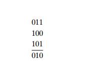
Since this sum contains a 1, the instance is a winning one for the player moving first. To find a winning move from this position, the player needs to change one of the three bit strings so that the new nim sum contains only 0’s. It is not difficult to see that the only way to accomplish this is to remove two chips from the first pile.

This ingenious solution to the game of Nim was discovered by Harvard math-ematics professor C. L. Bouton more than 100 years ago. Since then, mathemati-cians have developed a much more general theory of such games. An excellent account of this theory, with applications to many specific games, is given in the monograph by E. R. Berlekamp, J. H. Conway, and R. K. Guy [Ber03].

Exercises 4.5

          1.   a. If we measure an instance size of computing the greatest common divisor of m and n by the size of the second number n, by how much can the size decrease after one iteration of Euclid’s algorithm?

            Prove that an instance size will always decrease at least by a factor of two after two successive iterations of Euclid’s algorithm.

            2. Apply quickselect to find the median of the list of numbers 9, 12, 5, 17, 20, 30, 8.

            3. Write pseudocode for a nonrecursive implementation of quickselect.

            4. Derive the formula underlying interpolation search.

            5. Give an example of the worst-case input for interpolation search and show that the algorithm is linear in the worst case.

          .   a.  Find the smallest value of n for which log₂ log₂ n + 1 is greater than 6.

            Determine which, if any, of the following assertions are true:

i. log log n ∈ o(log n)                       ii. log log n ∈  (log n)     iii. log log n ∈  (log n)

            . a. Outline an algorithm for finding the largest key in a binary search tree. Would you classify your algorithm as a variable-size-decrease algorithm?

            What is the time efficiency class of your algorithm in the worst case?

            a. Outline an algorithm for deleting a key from a binary search tree. Would you classify this algorithm as a variable-size-decrease algorithm?

            What is the time efficiency class of your algorithm in the worst case?

            9. Outline a variable-size-decrease algorithm for constructing an Eulerian circuit in a connected graph with all vertices of even degrees.

          10.   Mis`ere one-pile Nim Consider the so-called misere` version of the one-pile Nim, in which the player taking the last chip loses the game. All the other conditions of the game remain the same, i.e., the pile contains n chips and on each move a player takes at least one but no more than m chips. Identify the winning and losing positions (for the player to move next) in this game.

         11.    a. Moldy chocolate Two players take turns by breaking an m × n chocolate bar, which has one spoiled 1 × 1 square. Each break must be a single straight line cutting all the way across the bar along the boundaries between the squares. After each break, the player who broke the bar last eats the piece that does not contain the spoiled square. The player left with the spoiled square loses the game. Is it better to go first or second in this game?

           b. Write an interactive program to play this game with the computer. Your program should make a winning move in a winning position and a random legitimate move in a losing position.

            12. Flipping pancakes There are n pancakes all of different sizes that are stacked on top of each other. You are allowed to slip a flipper under one of the pancakes and flip over the whole stack above the flipper. The purpose is to arrange pancakes according to their size with the biggest at the bottom. (You can see a visualization of this puzzle on the Interactive Mathematics Miscellany and Puzzles site [Bog].) Design an algorithm for solving this puzzle.

            13. You need to search for a given number in an n × n matrix in which every row and every column is sorted in increasing order. Can you design a O(n) algorithm for this problem? [Laa10]