Insertion Sort

Insertion Sort

In this section, we consider an application of the decrease-by-one technique to sorting an array A[0..n − 1]. Following the technique’s idea, we assume that the smaller problem of sorting the array A[0..n − 2] has already been solved to give us a sorted array of size n − 1: A[0] ≤ ^{. . .} ≤ A[n − 2]. How can we take advantage of this solution to the smaller problem to get a solution to the original problem by taking into account the element A[n − 1]? Obviously, all we need is to find an appropriate position for A[n − 1] among the sorted elements and insert it there. This is usually done by scanning the sorted subarray from right to left until the first element smaller than or equal to A[n − 1] is encountered to insert A[n − 1] right after that element. The resulting algorithm is called straight insertion sort or simply insertion sort.

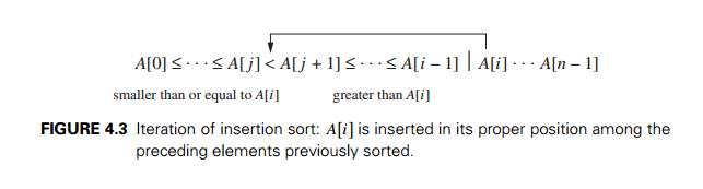
Though insertion sort is clearly based on a recursive idea, it is more efficient to implement this algorithm bottom up, i.e., iteratively. As shown in Figure 4.3, starting with A[1] and ending with A[n − 1], A[i] is inserted in its appropriate place among the first i elements of the array that have been already sorted (but, unlike selection sort, are generally not in their final positions).

Here is pseudocode of this algorithm.

ALGORITHM                 InsertionSort(A[0..n − 1])

//Sorts a given array by insertion sort

//Input: An array A[0..n − 1] of n orderable elements //Output: Array A[0..n − 1] sorted in nondecreasing order for i ← 1 to n − 1 do

v ← A[i] j ← i − 1

while j ≥ 0 and A[j ] > v do

A[j + 1] ← A[j ] j ← j − 1

A[j + 1] ← v

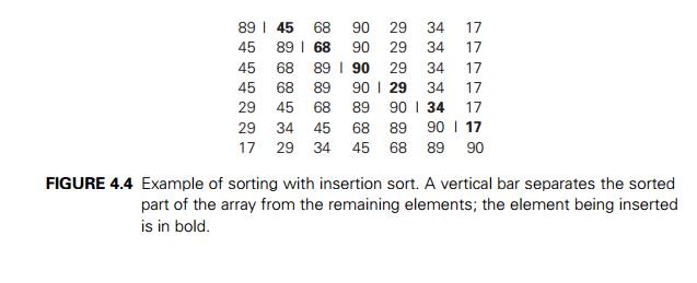
The operation of the algorithm is illustrated in Figure 4.4.

The basic operation of the algorithm is the key comparison A[j ] > v. (Why not j ≥ 0? Because it is almost certainly faster than the former in an actual computer implementation. Moreover, it is not germane to the algorithm: a better imple-mentation with a sentinel—see Problem 8 in this section’s exercises—eliminates it altogether.)

The number of key comparisons in this algorithm obviously depends on the nature of the input. In the worst case, A[j ] > v is executed the largest number of times, i.e., for every j = i − 1, . . . , 0. Since v = A[i], it happens if and only if A[j ] > A[i] for j = i − 1, . . . , 0. (Note that we are using the fact that on the ith iteration of insertion sort all the elements preceding A[i] are the first i elements in the input, albeit in the sorted order.) Thus, for the worst-case input, we get A[0] > A[1] (for i = 1), A[1] > A[2] (for i = 2), . . . , A[n − 2] > A[n − 1] (for i = n − 1). In other words, the worst-case input is an array of strictly decreasing values. The number of key comparisons for such an input is

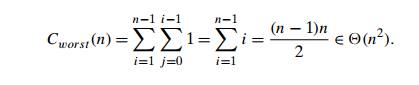
Thus, in the worst case, insertion sort makes exactly the same number of compar-isons as selection sort (see Section 3.1).

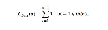
In the best case, the comparison A[j ] > v is executed only once on every iteration of the outer loop. It happens if and only if A[i − 1] ≤ A[i] for every i = 1, . . . , n − 1, i.e., if the input array is already sorted in nondecreasing order. (Though it “makes sense” that the best case of an algorithm happens when the problem is already solved, it is not always the case, as you are going to see in our discussion of quicksort in Chapter 5.) Thus, for sorted arrays, the number of key comparisons is

This very good performance in the best case of sorted arrays is not very useful by itself, because we cannot expect such convenient inputs. However, almost-sorted files do arise in a variety of applications, and insertion sort preserves its excellent performance on such inputs.

A rigorous analysis of the algorithm’s average-case efficiency is based on investigating the number of element pairs that are out of order (see Problem 11 in this section’s exercises). It shows that on randomly ordered arrays, insertion sort makes on average half as many comparisons as on decreasing arrays, i.e.,

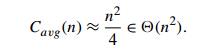
This twice-as-fast average-case performance coupled with an excellent efficiency on almost-sorted arrays makes insertion sort stand out among its principal com-petitors among elementary sorting algorithms, selection sort and bubble sort. In addition, its extension named shellsort, after its inventor D. L. Shell [She59], gives us an even better algorithm for sorting moderately large files (see Problem 12 in this section’s exercises).

Exercises 4.1

1. Ferrying soldiers A detachment of n soldiers must cross a wide and deep river with no bridge in sight. They notice two 12-year-old boys playing in a rowboat by the shore. The boat is so tiny, however, that it can only hold two boys or one soldier. How can the soldiers get across the river and leave the boys in joint possession of the boat? How many times need the boat pass from shore to shore?

2. Alternating glasses

            There are 2n glasses standing next to each other in a row, the first n of them filled with a soda drink and the remaining n glasses empty. Make the glasses alternate in a filled-empty-filled-empty pattern in the minimum number of glass moves. [Gar78]

            Solve the same problem if 2n glasses—n with a drink and n empty—are initially in a random order.

3. Marking cells Design an algorithm for the following task. For any even n, mark n cells on an infinite sheet of graph paper so that each marked cell has an odd number of marked neighbors. Two cells are considered neighbors if they are next to each other either horizontally or vertically but not diagonally. The marked cells must form a contiguous region, i.e., a region in which there is a path between any pair of marked cells that goes through a sequence of marked neighbors. [Kor05]

4. Design a decrease-by-one algorithm for generating the power set of a set of n elements. (The power set of a set S is the set of all the subsets of S, including the empty set and S itself.)

5. Consider the following algorithm to check connectivity of a graph defined by its adjacency matrix.

ALGORITHM     Connected(A[0..n − 1, 0..n − 1])

//Input: Adjacency matrix A[0..n − 1, 0..n − 1]) of an undirected graph G //Output: 1 (true) if G is connected and 0 (false) if it is not

if n = 1 return 1   //one-vertex graph is connected by definition

else

if not Connected(A[0..n − 2, 0..n − 2]) return 0 else for j ← 0 to n − 2 do

if A[n − 1, j ] return 1 return 0

Does this algorithm work correctly for every undirected graph with n > 0 vertices? If you answer yes, indicate the algorithm’s efficiency class in the worst case; if you answer no, explain why.

7.             Team ordering You have the results of a completed round-robin tournament in which n teams played each other once. Each game ended either with a victory for one of the teams or with a tie. Design an algorithm that lists the teams in a sequence so that every team did not lose the game with the team listed immediately after it. What is the time efficiency class of your algorithm?

8. Apply insertion sort to sort the list E, X, A, M, P , L, E in alphabetical order.

            a. What sentinel should be put before the first element of an array being sorted in order to avoid checking the in-bound condition j ≥ 0 on each iteration of the inner loop of insertion sort?

b. Is the sentinel version in the same efficiency class as the original version?

9. Is it possible to implement insertion sort for sorting linked lists? Will it have the same O(n²) time efficiency as the array version?

10. Compare the text’s implementation of insertion sort with the following ver-sion.

ALGORITHM     InsertSort2(A[0..n − 1])

for i ← 1 to n − 1 do j ← i − 1

while j ≥ 0 and A[j ] > A[j + 1] do swap(A[j ], A[j + 1])

j ← j – 1

What is the time efficiency of this algorithm? How is it compared to that of the version given in Section 4.1?

11. Let A[0..n − 1] be an array of n sortable elements. (For simplicity, you may assume that all the elements are distinct.) A pair (A[i], A[j ]) is called an inversion if i < j and A[i] > A[j ].

            What arrays of size n have the largest number of inversions and what is this number? Answer the same questions for the smallest number of inversions.

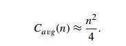
            Show that the average-case number of key comparisons in insertion sort is given by the formula

12. Shellsort (more accurately Shell’s sort) is an important sorting algorithm that works by applying insertion sort to each of several interleaving sublists of a given list. On each pass through the list, the sublists in question are formed by stepping through the list with an increment h_i taken from some predefined decreasing sequence of step sizes, h₁ > ^{. . .} > h_i > ^{. . .} > 1, which must end with 1. (The algorithm works for any such sequence, though some sequences are known to yield a better efficiency than others. For example, the sequence 1, 4, 13, 40, 121, . . . , used, of course, in reverse, is known to be among the best for this purpose.)

a.  Apply shellsort to the list

S, H, E, L, L, S, O, R, T , I, S, U, S, E, F, U, L

            Is shellsort a stable sorting algorithm?

            Implement shellsort, straight insertion sort, selection sort, and bubble sort in the language of your choice and compare their performance on random arrays of sizes 10ⁿ for n = 2, 3, 4, 5, and 6 as well as on increasing and decreasing arrays of these sizes.