Three Dimensional Display Methods

THREE DIMENSIONAL DISPLAY METHODS

To obtain display of a three-dimensional scene that has been modeled in world coordinates. we must first set up a coordinate reference for the "camera". This coordinate reference defines the position and orientation for the plane of the carnera film which is the plane we want to us to display a view of the objects in the scene. Object descriptions are then transferred to the camera reference coordinates and projected onto the selected display plane. We can then display the objects in wireframe (outline) form, or we can apply lighting surface rendering techniques to shade the visible surfaces.

 PARALLEL PROJECTION

In a parallel projection, parallel lines in the world-coordinate scene projected into parallel lines on the two-dimensional display plane.

 Perspective Projection

Another method for generating a view of a three-dimensional scene is to project points to the display plane along converging paths. This causes objects farther from the viewing position to be displayed smaller than objects of the same size that are nearer to the viewing position.In a perspective projection, parallel lines in a scene that are not parallel to the display plane are projected into converging lines

 DEPTH CUEING

A simple method for indicating depth with wireframe displays is to vary the intensity of objects according to their distance from the viewing position. The viewing position are displayed with the highest intensities, and lines farther away are displayed with decreasing intensities.

Visible Line and Surface Identification

We can also clarify depth relation ships in a wireframe display by identifying visible lines in some way. The simplest method is to highlight the visible lines or to display them in a different color. Another technique, commonly used for engineering drawings, is to display the nonvisible lines as dashed lines. Another approach is to simply remove the nonvisible lines

Surface Rendering

Added realism is attained in displays by setting the surface intensity of objects according to the lighting conditions in the scene and according to assigned surface characteristics. Lighting specifications include the intensity and positions of light sources and the general background illumination required for a scene. Surface properties of objects include degree of transparency and how rough or smooth the surfaces are to be. Procedures can then be applied to generate the correct illumination and shadow regions for the scene.

 Exploded and Cutaway View

Exploded and cutaway views of such objects can then be used to show the internal structure and relationship of the object Parts

Three-Dimensional and Stereoscopic View

Three-dimensional views can be obtained by reflecting a raster image from a vibrating flexible mirror. The vibrations of the mirror are synchronized with the display of the scene on the CRT. As the mirror vibrates, the focal length varies so that each point in the scene is projected to a position corresponding to its depth.

Stereoscopic devices present two views of a scene: one for the left eye and the other for the right eye.

THREE DIMENSIONAL OBJECT REPRESENTATIONS

Representation schemes for solid objects are often divided into two broad categories

Boundary representations (B-reps) describe a three-dimensional object as a set of surfaces that separate the object interior from the environment.Typical examples of boundary representations are polygon facets and spline patches.

Space-partitioning representations are used to describe interior properties, by partitioning the spatial region containing an object into a set of small, nonoverlapping, contiguous solids (usually cubes).

POLYGON SURFACES

The most commonly used boundary representation for a three-dimensional graphics object is a set of surface polygons that enclose the object interior. Many graphics systems store all object descriptions as sets of surface polygons. This simplifies and speeds up the surface rendering and display of objects, since all surfaces are described with linear equations. For this reason, polygon descriptions are often referred to as "standard graphics objects."

Polygon Tables

We specify a polygon surface with a set of vertex coordinates and associated attribute parameters. As information for each polygon is input, the data are placed into tables that are to be used in the subsequent' processing, display, and manipulation of the objects in a scene.

Polygon data tables can be organized into two groups:

geometric tables - attribute tables.

Geometric data tables contain vertex coordinates and parameters to identify the spatial orientation of the polygon surfaces.

Attribute information for an object includes parameters specifying the degree of transparency of the object and its surface reflectivity and texture characteristics.

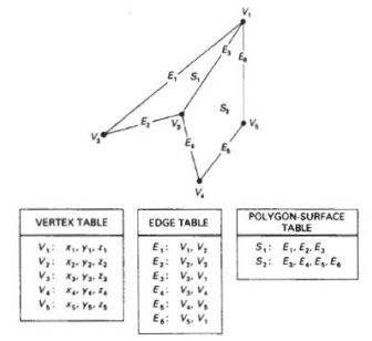
A convenient organization for storing geometric data is to create three lists: a vertex table, an edge

table, and a polygon table.

Coordinate values for each vertex in the object are stored in the vertex table. The edge table contains pointers back into the vertex table to identify the vertices for each polygon edge. And thepolygon table contains pointers back into the edge table to identify the edges for each polygon.

Plane Equations

To produce a display of a three-dimensional object, we must process the input data representation for the object through several procedures.

These processing steps include transformation of the modeling and world-coordinate descriptions to viewing coordinates, then to device coordinates; identification of visible surfaces; and the application of surface-rendering procedures.

The equation for 'I plane surface can be expressed In the form Ax + By + Cz + D =0

where (r, y, z ) is any point on the plane, and the coefficients A, B, C, and D are constants describing the spatial objects of the plane

we select three successive polygon vertices (x1, y1,z1), (x2, y2,z2), (x3, y3,z3),

and solve thc following set of simultaneous linear plane equation5 for the ratios AID, B/D,and ClD

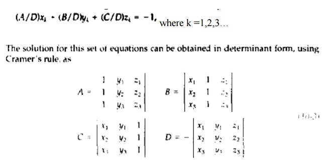
Expanding thc determinants, we can write the calculations for the plane coefficients in the form

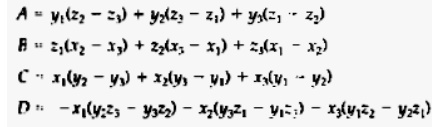
As vertex values and other information are entered into the polygon data structure,values tor A, B, C. and D are computed for each polygon and stored with the other polygon data.

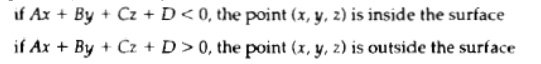
Plane equations are used also to identify the position of spatial points relativeto the plane surfaces of an object. For any point (x, y, z) not on a plane withparameters A, B, C, D, we have Ax + By+ Cz+ D != 0 We can identify the point as either inside or outside the plane surface accordingto the sign (negative or positive) of Ax + By + Cz + D:

CURVED LINES AND SURFACES

Curve and surface equations can be expressed in either a parametric or anonparametric form.

QUADRIC SURFACES

A frequently used class of objects is the quadric surfaces, which are described with second-degree equations (quadratics). They include spheres, ellipsoids, tori, paraboloids, and hyperboloids. Quadric surfaces, particularly spheres and ellipsoids, are common elements of graphics scenes.

Sphere

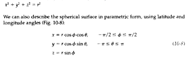
In Cartesian coordinates, a spherical surface with radius r centered on the coordi-nate origin is defined as the set of points (x, y, z) that satisfy the equation

Torus

A torus is a doughnut-shaped object, as shown in Fig. It can be generated by rotating a circle or other conic about a specified axis. The Cartesian representation for points over the surface of a torus can be written in the form

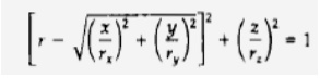
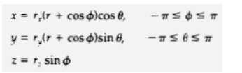
where r is any given offset value. Parametric representations for a torus are similar to those for an ellipse, except that angle d extends over 360". Using latitude and longitude angles , we can describe the toms surface as the set of points that satisfy

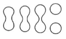
BLOBBY OBJECTS

Some objects do not maintain a fixed shape, but change their surface characteristics in certain motions or when in proximity to other opts.

Examples in this class of objects include molecular structures, water droplets and other liquid effects, melting objects, and muscle shapes in the human body. These objects can bedescribed as exhibiting "blobbiness" and are often simply referred to as blobby objects, since their shapes show a certain degree of fluidity.

Eg:

Surface function is then defined as

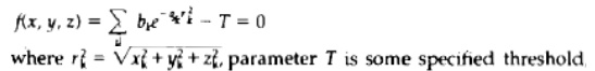
And a& b – to adjust the amount of blobbiness of an object.

SPLINE REPRESENTATIONS

In drafting terminology, a spline is a flexible strip used to produce a smoothcurve through a designated set of points. Several small weights are distributed along the length of the strip to hold it in position on the drafting table as the curve is drawn.

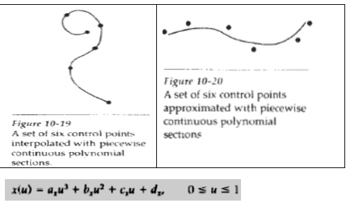
INTERPOLATION AND APPROXIMATION SPLINES

We specify a spline curver by giving a set of coordinate positions, called control points, which indicates the general shape of the curve. These control points are then fitted with piece wise continuous parametric poly nomial functions in one of two ways.

When polynomial sections are fitted so that the curve passes through

each control point, the resulting curve is said to interpolate the set of control points.

On the other hand, when the polynomials are fitted to the general control-point path without necessarily passing through any control point, the resulting curve is said to approximate the set of control points

Spline Specifications

There are three equivalent methods for specifying a particular spline representation:

(1) We can state the set of boundary conditions that are imposed on the spline;

(2)     we can state the matrix that characterizes the spline; or

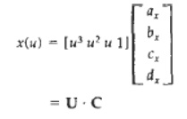
(3)     we can state the set of blending functions (or basis functions) that determine how specified geometric constraints on the curve are combined to calculate positions along the curve path we have the following parametric cubic polynomial representation for the x coordinate along the path of a spline section:

Boundary conditions for this curve might be set, for example, on the endpoint coordinates x(0) and x(l) and on the parametric first derivatives at the endpoints x'(0) and x' ( 1 ) . These four boundary conditions are sufficient to determine the values of the four coefficients ak, bk, ck, and dk.

=U.C

Where U – row matrix of powers of parameter u

C – coefficient column matrix

1.     To obtain a polynomial representation for coordinate x in terms of the geometric constraint parameters

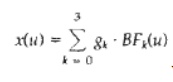
where gk are the constraint parameters, such as the control-point coordinates and slope of the curve at the control points, and BFk(u) are the polynomial blending functions.

BEZIER CURVES AND SURFACES

This spline approximation method was developed by the French engineer Pierre Mzier for use in the design of Renault automobile bodies. Bezier splines have a number of properties that make them highly useful and convenient for curve and surface design.

Bezier Curves

In general, a Bezier curve section can be fitted to any number of control points.

The number of control points to be approximated and their relative position determine the degree of the BCzier polynomial. As with the interpolation splines, a bezier curve can be specified with boundary conditions, with a characterizing matrix, or with blending functions.

For general Bezier curves, the blending-function specification is the most convenient.

Suppose we are given n + 1 control-point positions: pk = (xk, yk, zk), with k varying from 0 to n. These coordinate points can be blended to produce the following position vector P(u), which describes the path of an approximating Bezier polynomial function between p1, and p_n.

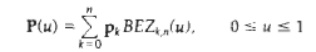
The Bezier blending functions BEZ_k,n,(u) are the Bemstein polynomials:

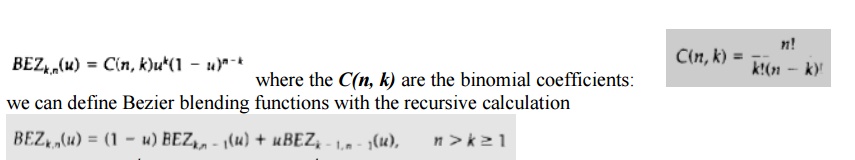
with BEZk,k = u^k, and BEZ_0.k= (1 - u ) ^k

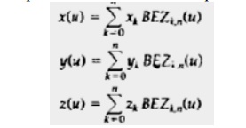
vector equation represents a set of three parametric equations for the individual curve coordinates

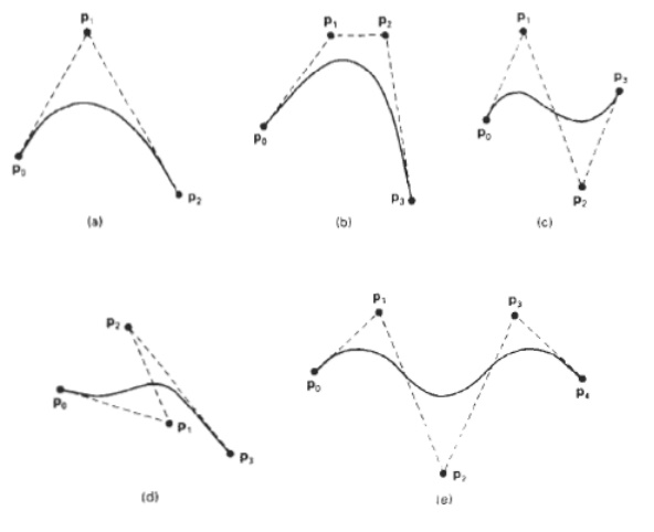
a Bezier curve is a polynomial of degree one less than the number of control points used: Three points generate a parabola, four points a cubiccurve, and so forth. For Example

Properties of Bezier Curves

1. A very useful property of a Bezier curve is that it always passes through the first and last control points. That is, the boundary conditions at the two ends of the curve are

2. Values of the parametric first derivatives of a Bezier curve at the endpoints can be calculated from control point coordinates as

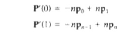
Thus, the slope at the beginning of the curve is along the line joining the first two control points, and the slope at the end of the curve is along the line joining the last two endpoints.

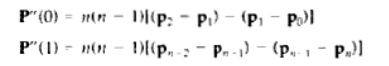
3. Similarly, the parametric second derivatives o f a Bezier curve at the endpoints are calculated as

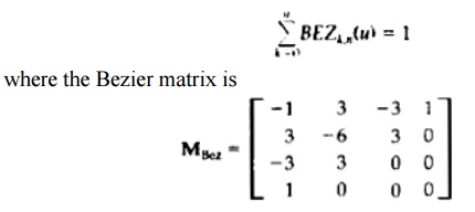
Another important property of any Bezier curve is that it lies within the convex hull (convex polygon boundary) of the control points. This follows from the properties of Bezier blending functions:

They are all positive and is always one.

Bezier Surtaces

Two sets of orthogonal Bezier curves can be used to design an object surface by specifying by an input mesh of control points. The parametric vector function for the Bezier surface is formed as the Cartesian product of Bezier blending functions:

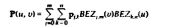
with Pj,k specifying the location of the (m + 1) by (n + I ) control points.

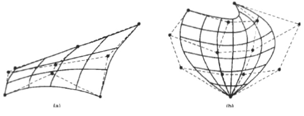
The control points are connected by dashed lines, and the solid lines show curves of constant u and constant v. Each curve of constant u is plotted by varying v over the interval from 0to 1, with u fixed at one of the values in this unit interval. Curves of constant v are plotted similarly

B-SPLINE CURVES AND SURFACES

B-splines have two advantages over Bezier splines:

(1) the degree of a B-spline polynomial can be set independently of the number of control points (with certain limitations),

(2) B-splines allow local control over the shape of a spline curve or surface

B-Spline Curves

We can write a general expression for the calculation of coordinate positions along a B-spline curve in a blending-function formulation as

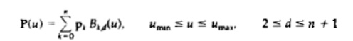
where the pk are an input set of n + 1 control points.

Blending functions for B-spline curves are defined by the Cox-deBoor recursion  formulas:

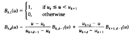
where each blendjng function is defined over d subintervals of the total range of u. The selected set of subinterval endpoints u, is referred to as a knot vector. B-spline curves have the following properties.

The polynomial curve has degree d - 1 and C^d-2 continuity over the rangeof u. For n + 1 control points, the curve is described with n + 1 blending functions.

Each blending function B_k,d, is defined over d subintervals of the total range of u, starting at knot value u1.

The range of parameter u 1s divided into n + d subintervals by the n + d +1 values specified in the knot vector.

With knot values labeled as [u1, u2, . . . , un,], the resulting B-spline curve is defined only in the interval from knot value u_d-1 , up to knot value u_n+1.

Each section of the spline curve (between two successive knot values) is influenced by d control points.

Any one control point can affect the shape of at most d curve sections.

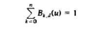
B-splines are tightly bound to the input positions. For any value of u in the interval from knot value u_d-1 to u_n+1 the sum over all basis functions is 1:

^Ø Uniform, Periodic B-Splines

When the spacing between knot values is constant, the resulting curve is called a uniform B-spline.

 ^ØCubic, Periodic B-Splines

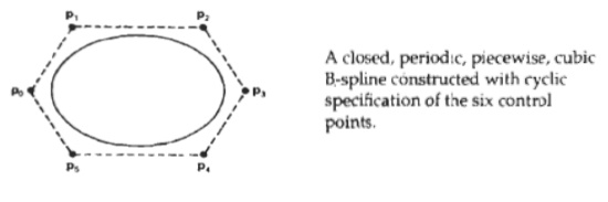
Since cubic, periodic 8-splines are commonly used in graphics packages, we consider the fornlulation for this class of splines. Periodic splines are particularly useful for generating certain closed curves

^Ø Open Uniform B-Splines

This class of B-splines is a cross between uniform B-splines and nonuniform Bsplines. Sometimes it is treated as a special type of uniform 8-spline, and sometimes it is considered to be in the nonuniform B-splines classification.

For the open uniform B-splines, or simply open B-splines, the knot spacing is uniform except at the ends where knot values are repeated d times.

For any values of parameters d and n, we can generate an open uniform knot vector with integer values using the calculations

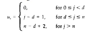
for values of] ranging from 0 to n + d. With this assignment, the first d knots are assigned the value 0, and the last d knots have the value n - d + 2.

^Ø Non Uniform B-Splines

For this class of splines, we can specify any values and intervals for the knot vector. With nonuniform B-splines, we can choose multiple internal knot values and unequal spacing between the knot values.

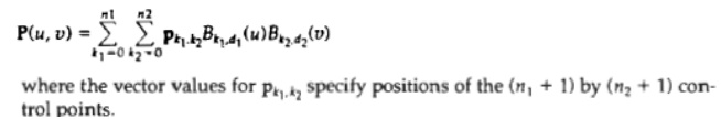
B-Spline Surfaces

We can obtain a vector point function over a B-spline surface using the Cartesian product ofB-spline blending functions in the form

OCTREES

Hierarchical tree structures, called octrees, are used to represent solid objects in some graphics systems.The tree structure is organized so that each node corresponds to a region of three-dimensional space. This representation for solids takes advantage of spatial coherence to reduce storage requirements for three-dimensional objects. It also provides a convenient representation for storing information about object interiors.

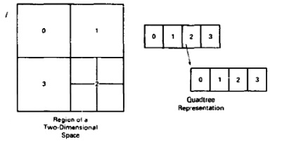
The octree encoding procedure for a three-dimensional space is an extensionof an encoding scheme for two-dimensional space, called quadtree encoding.Quadtrees are generated by successively dividing a two-dimensional region (usually a square) into quadrants. Each node in the quadtree has four data elements,one for each of the quadrants in the region

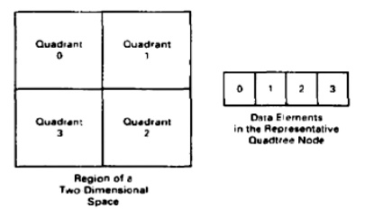
If all pixels within a quadrant have the same color (a homogeneous quadrant), the corresponding data element in the node stores that color.

In addition, a flag is set in the data element to indicate that the quadrant is homogeneous. Suppose all pixels in quadrant are found to be red. The color code for red is then placed in data element 2 of the node. Otherwise, the quadrant is said to be heterogeneous, and that quadrant is itself divided into quadrants

An octree encoding scheme divides regions of three-dimensional space (usually cubes) into octants and stores eight data elements in each node of the tree

Individual elements of a three-dimensional space are called volume elements, or voxels.

When all voxels in an octant are of the same type this type value is stored in the corresponding data element of the node..

Empty regions of space are represented by voxel type "void."

Any heterogeneous octant is subdivided into octants, and the corresponding data element in the node points to the next node in the octree.

BSP TREES

This representation scheme is similar to octree encoding, except we now divide space into two partitions instead of eight at each step.

With a binary space-partitioning (BSP) tree, we subdivide a scene into two sections at each step with aplane that can be at any position and orientation.

In an octree encoding, the scene is subdivided at each step with three mutually perpendicular planes aligned with the Cartesian coordinate planes.