The Principal Sources of Optimization

The Principal Sources of Optimization

1 Causes of Redundancy

2 A Running Example: Quicksort

3 Semantics-Preserving Transformations

4 Global Common Subexpressions

5 Copy Propagation

6 Dead-Code Elimination

7 Code Motion

8 Induction Variables and Reduction in Strength

9 Exercises for Section 9.1

A compiler optimization must preserve the semantics of the original program. Except in very special circumstances, once a programmer chooses and imple-ments a particular algorithm, the compiler cannot understand enough about the program to replace it with a substantially different and more efficient al-gorithm. A compiler knows only how to apply relatively low-level semantic transformations, using general facts such as algebraic identities like i + 0 = i or program semantics such as the fact that performing the same operation on the same values yields the same result.

1. Causes of Redundancy

There are many redundant operations in a typical program. Sometimes the redundancy is available at the source level. For instance, a programmer may find it more direct and convenient to recalculate some result, leaving it to the compiler to recognize that only one such calculation is necessary. But more often, the redundancy is a side effect of having written the program in a high-level language. In most languages (other than C or C + + , where pointer arithmetic is allowed), programmers have no choice but to refer to elements of an array or fields in a structure through accesses like A[i][j] or X -+ fl.

As a program is compiled, each of these high-level data-structure accesses expands into a number of low-level arithmetic operations, such as the computation of the location of the (i, j ) t h element of a matrix A. Accesses to the same data structure often share many common low-level operations. Programmers are not aware of these low-level operations and cannot eliminate the redundancies themselves. It is, in fact, preferable from a software-engineering perspective that programmers only access data elements by their high-level names; the programs are easier to write and, more importantly, easier to understand and evolve. By having a compiler eliminate the redundancies, we get the best of both worlds: the programs are both efficient and easy to maintain.

2. A Running Example: Quicksort

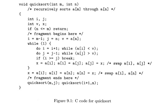
In the following, we shall use a fragment of a sorting program called quicksort to illustrate several important code-improving transformations. The C program in Fig. 9.1 is derived from Sedgewick,¹ who discussed the hand-optimization of such a program. We shall not discuss all the subtle algorithmic aspects of this program here, for example, the fact that a[0) must contain the smallest of the sorted elements, and a[max] the largest.

Before we can optimize away the redundancies in address calculations, the address operations in a program first must be broken down into low-level arith-metic operations to expose the redundancies. In the rest of this chapter, we as-sume that the intermediate representation consists of three-address statements, where temporary variables are used to hold all the results of intermediate ex-pressions. Intermediate code for the marked fragment of the program in Fig. 9.1 is shown in Fig. 9.2.

In this example we assume that integers occupy four bytes. The assignment x = a [ i ] is translated as in Section 6.4.4 into the two three-address statements

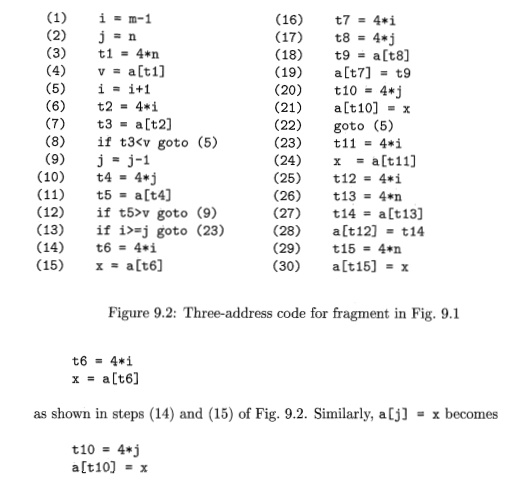
in steps (20) and (21). Notice that every array access in the original program translates into a pair of steps, consisting of a multiplication and an array-subscripting operation. As a result, this short program fragment translates into a rather long sequence of three-address operations.

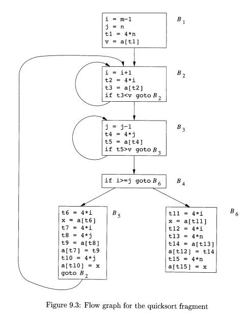
Figure 9.3 is the flow graph for the program in Fig. 9.2. Block B1 is the entry node. All conditional and unconditional jumps to statements in Fig. 9.2 have been replaced in Fig. 9.3 by jumps to the block of which the statements are leaders, as in Section 8.4. In Fig. 9.3, there are three loops. Blocks B₂ and JE?3 are loops by themselves. Blocks B₂, B₃, B±, and B$ together form a loop, with B₂ the only entry point.

3. Semantics-Preserving Transformations

There are a number of ways in which a compiler can improve a program without changing the function it computes. Common-subexpression elimination, copy propagation, dead-code elimination, and constant folding are common examples of such function-preserving (or semantics-preserving) transformations; we shall consider each in turn.

Frequently, a program will include several calculations of the same value, such as an offset in an array. As mentioned in Section 9.1.2, some of these duplicate calculations cannot be avoided by the programmer because they lie below the level of detail accessible within the source language. For example, block £5 shown in Fig. 9.4(a) recalculates 4 * i and 4* j, although none of these calculations were requested explicitly by the programmer.

4. Global Common Subexpressions

An occurrence of an expression E is called a common subexpression if E was previously computed and the values of the variables in E have not changed since the previous computation. We avoid recomputing E if we can use its previously computed value; that is, the variable x to which the previous computation of E was assigned has not changed in the interim.

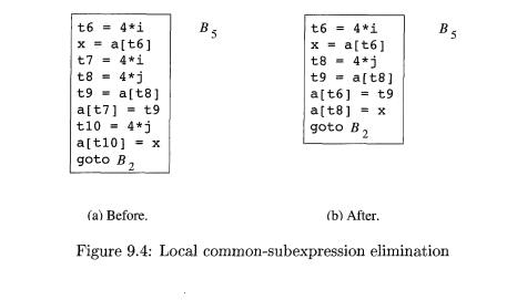
Example 9 . 1 : The assignments to t7 and t l O in Fig. 9.4(a) compute the common subexpressions 4 * i and 4 * j, respectively. These steps have been eliminated  in Fig.  9.4(b), which uses t6 instead of t7 and t8 instead of t l O .

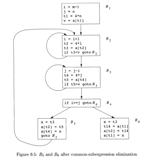
Example  9.2 :  Figure 9.5 shows the result of eliminating both global and local common subexpressions from blocks f?5 and BQ in the flow graph of Fig. 9.3. We first discuss the transformation of B5 and then mention some subtleties involving arrays.

After local common subexpressions are eliminated, B§ still evaluates 4*i and 4* j, as shown in Fig. 9.4(b). Both are common subexpressions; in particular, the three statements

2 If x has changed, it may still be possible to reuse the computation of E if we assign its value to a new variable y, as well as to x, and use the value of y in place of a recomputation of E.

using t4 computed in block B3.  In Fig. 9.5, observe that as control passes from the evaluation of 4 * j  in  B3    to B5, there is no change to j  and no change to £4, so t4 can be used if 4  * j  is needed.  

Another common  subexpression comes to light in  B5  after £4 replaces t8.

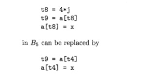
The new expression a[t4] corresponds to the value of a[j] at the source level. Not only does j retain its value as control leaves B3 and then enters f?5, but a[j], a value computed into a temporary t5, does too, because there are no assignments to elements of the array a in the interim. The statements

t 9  =  a [ t 4 ]

a [ t 6 ]  =  t 9

in B5 therefore can be replaced by

a [ t 6 ] = t 5

Analogously, the value assigned to x in block B₅ of Fig. 9.4(b) is seen to be the same as the value assigned to t3 in block B₂. Block B₅ in Fig. 9.5 is the result of eliminating common subexpressions corresponding to the values of the source level expressions a[i] and a[j] from B₅ in Fig. 9.4(b). A similar series of transformations has been done to BQ in Fig. 9.5.

The expression a[tl] in blocks B1 and B6 of Fig. 9.5 is not considered a  common subexpression, although tl can be used in both places. After control  leaves B1 and before it reaches B6, it can go through B5, where there are  assignments to a. Hence, a[tl] may not have the same value on reaching B6 as  it did on leaving B1, and it is not safe to treat a[tl] as a common subexpression. 

5. Copy Propagation

Block B$ in Fig. 9.5 can be further improved by eliminating x, using two new transformations. One concerns assignments of the form u = v called copy state-ments, or copies for short. Had we gone into more detail in Example 9.2, copies would have arisen much sooner, because the normal algorithm for eliminating common subexpressions introduces them, as do several other algorithms.

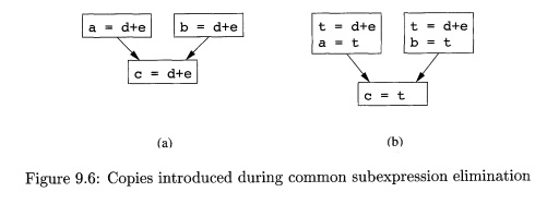
Example 9 . 3 :  In order to eliminate the common subexpression from the statement c  = d+e in Fig. 9.6(a), we must use a new variable t to hold the value of d + e. The value of variable t, instead of that of the expression d + e, is assigned to c in Fig. 9.6(b).  Since control may reach c =  d+e either after the assignment to a or after the assignment to b, it would be incorrect to replace c  =  d+e by either c  = a or by c =  b.

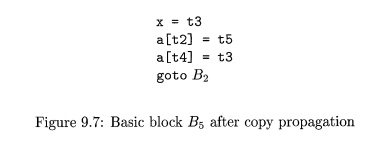
The  idea behind  the  copy-propagation transformation  is  to  use  v  for  ii, wherever possible after the copy statement u  = v.  For example, the assignment x  =  t3 in block B5   of Fig. 9.5 is a copy.  Copy propagation applied to B$ yields the code in Fig. 9.7. This change may not appear to be an improvement, but, as we shall see in Section 9.1.6, it gives us the opportunity to eliminate the assignment to x.

6. Dead-Code Elimination

A variable is live at a point in a program if its value can be used subsequently; otherwise, it is dead at that point. A related idea is dead (or useless) code — statements that compute values that never get used. While the programmer is unlikely to introduce any dead code intentionally, it may appear as the result of previous transformations.

E x a m p l e 9 . 4 : Suppose debug is set to TRUE or FALSE at various points in the program, and used in statements like

i f       (debug)        p r i n t      . . .

It may be possible for the compiler to deduce that each time the program reaches this statement, the value of debug is FALSE. Usually, it is because there is one particular statement

debug = FALSE

that must be the last assignment to debug prior to any tests of the value of debug, no matter what sequence of branches the program actually takes. If copy propagation replaces debug by FALSE, then the print statement is dead because it cannot be reached. We can eliminate both the test and the print operation from the object code. More generally, deducing at compile time that the value of an expression is a constant and using the constant instead is known as constant folding.

One advantage of copy propagation is that it often turns the copy statement into dead code. For example, copy propagation followed by dead-code elimination removes the assignment to x and transforms the code in Fig 9.7 into

a[t2]  = t5

a[t4]  = t3

goto B2

This code is a further improvement of block B5 in Fig. 9.5.

7. Code Motion

Loops are a very important place for optimizations, especially the inner loops where programs tend to spend the bulk of their time. The running time of a program may be improved if we decrease the number of instructions in an inner loop, even if we increase the amount of code outside that loop.

An important modification that decreases the amount of code in a loop is code motion. This transformation takes an expression that yields the same result independent of the number of times a loop is executed (a loop-invariant computation) and evaluates the expression before the loop. Note that the notion "before the loop" assumes the existence of an entry for the loop, that is, one basic block to which all jumps from outside the loop go (see Section 8.4.5).

Example 9 . 5 : Evaluation of limit — 2 is a loop-invariant computation in the following while-statement:

while  (i  <= limit-2)  /*  statement does not  change limit  */

Code motion will result in the equivalent code

t  =  limit-2

while  (i  <= t)      /*  statement does not  change limit  or t  */

Now, the computation of limit — 2 is performed once, before we enter the loop. Previously, there would be n +1 calculations of limit— 2 if we iterated the body of the loop n times. •

8. Induction Variables and Reduction in Strength

Another important optimization is to find induction variables in loops and optimize their computation. A variable x is said to be an. "induction variable" if there is a positive or negative constant c such that each time x is assigned, its value increases by c. For instance, i and tl are induction variables in the loop containing B₂ of Fig. 9.5. Induction variables can be computed with a single increment (addition or subtraction) per loop iteration. The transformation of replacing an expensive operation, such as multiplication, by a cheaper one, such as addition, is known as strength reduction. But induction variables not only allow us sometimes to perform a strength reduction; often it is possible to eliminate all but one of a group of induction variables whose values remain in lock step as we go around the loop.

When processing loops, it is useful to work "inside-out"; that is, we shall start with the inner loops and proceed to progressively larger, surrounding loops. Thus, we shall see how this optimization applies to our quicksort example by beginning with one of the innermost loops:  B 3   by itself. Note that the values of j and £4 remain in lock step; every time the value of j decreases by 1, the value of t4 decreases by 4, because 4 * j is assigned to t4. These variables, j and t4, thus form a good example of a pair of induction variables.

When there are two or more induction variables in a loop, it may be possible to get rid of all but one. For the inner loop of B₃ in Fig. 9.5, we cannot get rid of either j or t4 completely; t4 is used in B₃ and j is used in B±. However, we can illustrate reduction in strength and a part of the process of induction-variable elimination. Eventually, j will be eliminated when the outer loop consisting of blocks B?,,B₃,B± and B5 is considered.

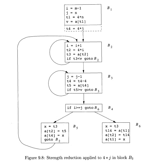
Example 9 . 6 :  As the relationship £4 = 4 * j surely holds after assignment to £4 in Fig. 9.5, and £4 is not changed elsewhere in the inner loop around B3, it follows that just  after the statement j = j - 1 the relationship £4 = 4 * j + 4 must hold. We may therefore replace the assignment t4 = 4* j by t4 = t 4 - 4 . The only problem is that £4 does not have a value when we enter block B3 for the first time.

Since we must maintain the relationship £4 = 4 * j on entry to the block B3, we place an initialization of £4 at the end of the block where j itself is initialized, shown by the dashed addition to block B1 in Fig. 9.8. Although we have added one more instruction, which is executed once in block Bi, the replacement of a multiplication by a subtraction will speed up the object code if multiplication takes more time than addition or subtraction, as is the case on many machines.

We conclude this section with one more instance of induction-variable elimination. This example treats i and j in the context of the outer loop containing B2, B3, B4, and B5.

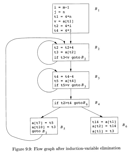
Example 9 . 7 : After reduction in strength is applied to the inner loops around B2 and B3, the only use of i and j  is to determine the outcome of the test in block B4.  We know that the values of i and t2 satisfy the relationship t2 = 4*i, while those of j and £4 satisfy the relationship ti = 4* j.  Thus, the test t2 > t1 can substitute for i > j.  Once this replacement is made, i in block B2   and j in block B3    become dead variables, and the assignments to them in these blocks become dead code that can be eliminated.  The resulting flow graph is shown in Fig. 9.9.

The code-improving transformations we have discussed have been effective. In Fig. 9.9, the numbers of instructions in blocks B₂ and B₃ have been reduced from 4 to 3, compared with the original flow graph in Fig. 9.3. In B₅, the number  has been reduced from 9 to 3, and in B₆ from 8 to 3. True, B1 has grown from four instructions to six, but Bi is executed only once in the fragment, so the total running time is barely affected by the size of B1.

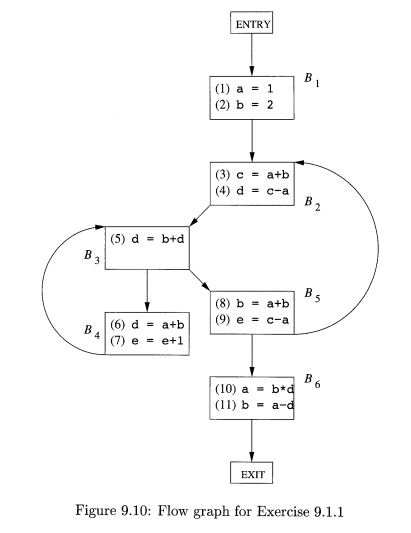
9. Exercises for Section 9 . 1

E x e r c i se 9 . 1 . 1 :  For the flow graph in Fig. 9.10:

            Identify the loops of the flow graph.

            Statements (1) and (2) in B1 are both copy statements, in which a and b are given constant values. For which uses of a and b can we perform copy propagation and replace these uses of variables by uses of a constant? Do so, wherever possible.

            Identify any global common subexpressions for each loop.

            Identify any induction variables for each loop. Be sure to take into account any constants introduced in (b).

            Identify any loop-invariant computations for each loop.

Exercise 9 . 1 . 2: Apply the transformations of this section to the flow graph

of Fig. 8.9.

Exercise 9 . 1 . 3 : Apply the transformations of this section to your flow graphs from (a) Exercise 8.4.1; (b) Exercise 8.4.2.

Exercise 9 . 1 . 4: In Fig. 9.11 is intermediate code to compute the dot product of two vectors A and B. Optimize this code by eliminating common subexpres-sions, performing reduction in strength on induction variables, and eliminating all the induction variables you can.

dp  = 0.

            = 0

            tl =  i*8

t2 = A[tl]

t3 =  i*8

t4 = B[t3]

t5 = t2*t4

dp = dp+t5 i = i +1

i f i <n  goto L

Figure 9.11:  Intermediate code to compute the dot product