Chapter: Compilers : Principles, Techniques, & Tools : Machine-Independent Optimizations
Region-Based Analysis
Region-Based Analysis
1 Regions
2 Region Hierarchies for Reducible Flow Graphs
3 Overview of a Region-Based Analysis
4 Necessary Assumptions About Transfer Functions
5 An Algorithm for Region-Based Analysis
6 Handling Nonreducible Flow Graphs
7 Exercises for Section 9.7
T he iterative data-flow analysis algorithm we have discussed so far is
just one approach to solving data-flow problems. Here we discuss another
approach called region-based analysis.
Recall that in the iterative-analysis approach, we create transfer functions
for basic blocks, then find the fixedpoint solution by repeated passes over the
blocks. Instead of creating transfer functions just for individual blocks, a
region-based analysis finds transfer functions that summa-rize the execution of
progressively larger regions of the program. Ultimately, transfer functions for
entire procedures are constructed and then applied, to get the desired
data-flow values directly.
While a data-flow framework using an iterative algorithm is specified by
a semilattice of data-flow values and a family of transfer functions closed
un-der composition, region-based analysis requires more elements. A
region-based framework includes both a semilattice of data-flow values and a
semilattice of transfer functions that must possess a meet operator, a
composition oper-ator, and a closure operator. We shall see what all these
elements entail in Section 9.7.4.
A region-based analysis is particularly useful for data-flow problems
where paths that have cycles may change the data-flow values. The closure
operator allows the effect of a loop to be summarized more effectively than
does iterative analysis. The technique is also useful for interprocedural
analysis, where trans-fer functions associated with a procedure call may be
treated like the transfer functions associated with basic blocks.
For simplicity, we shall consider only forward data-flow problems in
this section. We first illustrate how region-based analysis works by using the
familiar example of reaching definitions. In Section 9.8 we show a more
compelling use of this technique, when we study the analysis of induction
variables.
1. Regions
In region-based analysis, a program is viewed as a hierarchy of regions, which are (roughly) portions of
a flow graph that have only one point of entry. We should find this concept of
viewing code as a hierarchy of regions intuitive, because a block-structured
procedure is naturally organized as a hierarchy of regions. Each statement in a
block-structured program is a region, as control flow can only enter at the
beginning of a statement. Each level of statement nesting corresponds to a
level in the region hierarchy.
Formally, a region of a flow
graph is a collection of nodes N and
edges E such that
1. There is a header h in N that dominates all the nodes in N.
2. If some node m can reach a node n in N without going through h, then
m is also in N.
3. E is the set of all the control flow edges between nodes n1 and n2 in
N, except (possibly) for some that enter h.
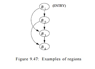
Example 9 . 5 0 : Clearly a natural loop is a region, but a region does
notnecessarily have a back edge and need not contain any cycles. For example,
in Fig. 9.47, nodes B1 and B2, together with the edge B1 —> B2: form a
region; so do nodes Bi,B2, and B3 with edges Bx B2, B2 ->• B3, and Bi ->
B3.
However, the subgraph with nodes
B2 and #3 with edge B2 —> B3 does not form a region, because control may
enter the subgraph at both nodes B2 and B3. More precisely, neither B2 nor B3 dominates
the other, so condition (1) for a region is violated. Even if we picked, say,
B2 to be the "header," we would violate condition (2), since we can
reach B3 from B1 without going through B2, and J5i is not in the
"region."
2. Region Hierarchies for
Reducible Flow Graphs
In what follows, we shall assume the flow graph is reducible. If
occasionally we must deal with nonreducible flow graphs, then we can use a
technique called "node splitting" that will be discussed in Section 9.7.6.
To construct a hierarchy of regions, we identify the natural loops.
Recall from Section 9.6.6 that in a reducible flow graph, any two natural loops
are either disjoint or one is nested within the other. The process of
"parsing" a reducible flow graph into its hierarchy of loops begins
with every block as a region by itself. We call these regions leaf regions. Then, we order the natural
loops from the inside out, i.e., starting with the innermost loops. To process
a loop, we replace the entire loop by a node in two steps:
1. First, the body of the loop
L (all nodes and edges except the
back edges to the header) is replaced by a node representing a region R. Edges to the header of L now enter the node for R. An edge from any exit of loop L is replaced by an edge from R to the same destination. However, if
the edge is a back edge, then it becomes a loop on R. We call R a body region.
2. Next, we construct a region R'
that represents the entire natural loop L.
We call R' a loop region. The only difference between R and R' is that the
latter includes the back edges to the header of loop L. Put another way, when R'
replaces R in the flow graph, all we
have to do is remove the edge from R
to itself.
We proceed this way, reducing larger and larger loops to single nodes,
first with a looping edge and then without. Since loops of a reducible flow
graph are nested or disjoint, the loop region's node can represent all the
nodes of the natural loop in the series of flow graphs that are constructed by
this reduction process.
Eventually, all natural loops are reduced to single nodes. At that
point, the flow graph may be reduced to a single node, or there may be several
nodes remaining, with ho loops; i.e., the reduced flow graph is an acyclic graph
of more than one node. In the former case we are done constructing the region
hierarchy, while in the latter case, we construct one more body region for the
entire flow graph.
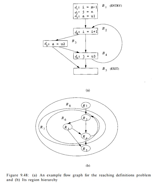
E x a m p l e 9 . 5 1 : Consider the control flow graph in Fig. 9.48(a).
There is one back edge in this flow graph, which leads from B4 to B2. The hierarchy of regions is shown in Fig. 9.48(b); the edges shown are
the edges in the region flow graphs. There are altogether 8 regions:
Regions Ri,... ,R& are leaf regions representing blocks B1 through B$, respectively. Every block is also an exit block in its region.
Body region RQ represents the body of the only loop in the flow graph;
it consists of regions R2,R3, and R4 and three interregion edges: B2 -»
B3, B2 -» BA, and B3
-> J54 . It has two exit blocks, B3
and £?4 , since they both have outgoing edges not contained in the
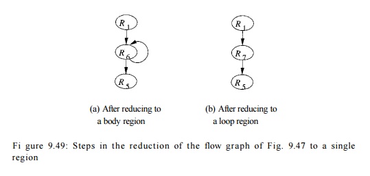
region. Figure 9.49(a) shows the flow graph with R$ reduced to a single node. Notice that although the edges R3 -> R5 and R4 -» -R5 have both been replaced by edge RQ
-» #5, it is important to remember that the latter edge represents the two
former edges, since we shall have to propagate transfer functions across this
edge eventually, and we need to know that what comes out of both blocks B3 and B4 will reach the header
of R$.
3. Loop region R7 represents the
entire natural loop. It includes one
subregion, RQ, and one back edge B4
-> B2. It has also two exit nodes, again B3 and B4.
Figure 9.49(b) shows the flow graph after the entire natural loop is
reduced to R7.
4. Finally, body region R8 is
the top region. It includes three regions, R±, R7, R5
and three interregion edges, B1 -> B2, B3
-» B5, and B4 B5. When we reduce the flow graph to R8,
it becomes a single node. Since there are no back edges to its header, B±,
there is no need for a final step reducing this body region to a loop region.
To summarize the process of decomposing reducible flow graphs
hierarchically, we offer the following algorithm.
Algorithm 9 . 5 2 : Constructing a bottom-up order of regions of a
reducible flow graph.
INPUT : A reducible flow graph G.
OUTPUT : A list of regions of G
that can be used in region-based data-flow problems.
METHOD :
Begin the list with all the leaf
regions consisting of single blocks of G,
in any order.
Repeatedly choose a natural loop L such that if there are any natural
loops contained within L, then these
loops have had their body and loop regions added to the list already. Add first
the region consisting of the
body of L (i.e., L without the back edges to the header
of L), and then the loop region of L.
If the entire flow graph is not
itself a natural loop, add at the end of the list the region consisting of the
entire flow graph.
3. Overview
of a Region-Based Analysis
For each region R, and for
each subregion R' within R, we compute a transfer function
/RJNIJ?'] that summarizes the effect of executing all possible paths
Where "Reducible" Comes
From
We now see why reducible flow graphs were given that name. While we
shall not prove this fact, the definition of "reducible flow graph"
used in this book, involving the back edges of the graph, is equivalent to
several definitions in which we mechanically reduce the flow graph to a single
node. The process of collapsing natural loops described in Section 9.7.2 is one
of them. Another interesting definition is that the reducible flow graphs are all
and only those graphs that can be reduced to a single node by the following two
transformations:
T11 Remove an
edge from a node to itself.
T2: If node n has a single
predecessor m, and n is not the entry
of the flow graph, combine m and n.
leading from the entry of R to
the entry of R', while staying within
R. We say that a block B within R is an exit block of
region R if it has an outgoing edge
to some block outside R. We also
compute a transfer function for each exit block B of R, denoted / f t , o U T [
. B ] > that summarizes the effect of executing all possible paths within R,
leading from the entry of R to the exit of B.
We then proceed up the region hierarchy, computing transfer functions
for progressively larger regions. We begin with regions that are single blocks,
where is,IN[13] is J u s t fn e identity function and / B 5 0UT [ B ] i s
the transfer function for the
block B itself. As we move up the
hierarchy,
• If R is a
body region, then the
edges belonging to R form an
acyclic graph on the subregions of R.
We may proceed to compute the transfer functions in a topological order
of the subregions.
If R is a loop region, then we only need to account for the effect of
the back edges to the header of R.
Eventually, we reach the top of the hierarchy and compute the transfer
functions for region Rn that is the entire flow graph. How we perform each of these
computations will be seen in Algorithm 9.53.
The next step is to compute the data-flow values at the entry and exit
of each block. We process the regions in the reverse order, starting with
region Rn and working our way down the hierarchy. For each region, we compute the data-flow values at the entry. For
region Rn, we apply /#n ) iN[.R] (IN[ENTRY]) to get the data-flow values at the entry of the
subregions R in Rn. We
repeat until we reach the basic blocks at the leaves of the region hierarchy.
4. Necessary Assumptions About
Transfer Functions
In order for region-based analysis to work, we need to make certain
assumptions about properties of the set of transfer functions in the framework.
Specifically, we need three primitive operations on transfer functions:
composition, meet and closure; only the first is required for data-flow
frameworks that use the iterative algorithm.
Composition
The transfer function of a sequence of nodes can be derived by composing
the functions representing the individual nodes. Let /i and f2 be transfer functions of nodes n1
and n2. The effect of executing n1
followed by n2 is represented by f2 o /]_. Function composition
has been discussed in Section 9.2.2, and an example using reaching definitions
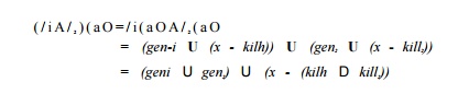
was shown in Section 9.2.4. To review, let gerii
and kilk be the gen and kill sets for Then:
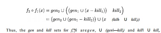
respectively. The same idea works for any transfer function of the
gen-kill form. Other transfer functions may also be closed, but we have to
consider each case separately.
Meet
Here, the transfer functions themselves are values of a semilattice with
a meet operator A/. The meet of two transfer functions f1 and f2, /i A/ f2, is
defined by (/i A/ fi){x)
= fi(x) A f2(x), where A
is the meet
operator for data-flow values.
The meet operator on transfer functions is used to combine the effect of
alternative paths of execution with the same end points. Where it is not
am-biguous, from now on, we shall refer to the meet operator of transfer
functions also as A. For the reaching-definitions framework, we have
That is, the
gen and kill
sets for f1 A f2 are gen1 U gen2
and killi n
kill2, respectively. Again, the same argument applies to any set of
gen-kill transfer functions.
Closure
If / represents the transfer function of a cycle, then fn represents the effect of going around the cycle n times. In the case where the number of iterations is not known,
we have to assume that the loop may be executed 0 or more times. We represent
the transfer function of such a loop by /*, the closure of /, which is defined by
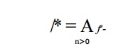
Note that /° must be the identity transfer function, since it represents
the effect of going zero times around the loop, i.e., starting at the entry and
not moving. If we let / represent the identity transfer function, then we can
write
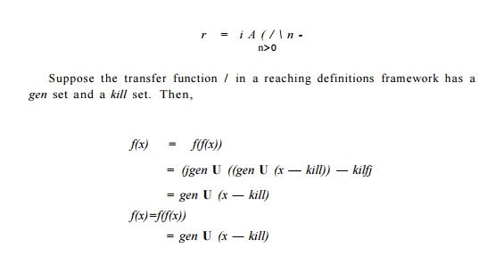
and so on: any fn(x) is gen U (x — kill). That is,
going around a loop doesn't affect the transfer function, if it is of the gen-kill form. Thus,
That is, the gen and kill sets for /* are gen and 0, respectively. Intuitively,
since we might not go around a ioop at all, anything in x will reach the entry to the loop. In all subsequent iterations,
the reaching definitions include those in the gen set.
5. An Algorithm for Region-Based
Analysis
T he following algorithm solves a
forward data-flow-analysis problem on a
reducible flow graph, according to some framework that satisfies the
assumptions of Section 9.7.4. Recall
that / R J N ^ ' ] and /j^ouTps] refer to
transfer functions that transform data-flow values at the entry to
region R into the correct value at the entry of subregion R' and the exit of
the exit block B, respectively.
Algorithm 9 . 5 3 : Region-based
analysis.
INPUT : A data-flow framework with the properties outlined in Section
9.7.4 and a reducible flow graph G.
OUTPUT : Data-flow values m[B] for each block B of G.
METHOD :
1. Use
Algorithm 9.52 to construct the bottom-up sequence of regions of G, say Ri,
R2,... ,Rn, where Rn is the topmost region.
2.
Perform the bottom-up analysis to compute the transfer functions sum-marizing
the effect of executing a region. For each region Ri, R2,... ,Rn, in the
bottom-up order, do the following:
(a) If R is a leaf region corresponding to block
B, let /RJN[ . B] — a n d
/ H , OUT
[ B ] = / B ,
the transfer function associated with block B.
If R is a
body region, perform the computation of Fig. 9.50(a).
If R is a
loop region, perform the computation of Fig. 9.50(b).
Perform the top-down pass to find the data-flow
values at the beginning of each region.
(a) w[Rn] = IN[ENTRY] .
(b) For each region R in {Ri,... Rn-i}, in the
top-down order, compute
I N [ J R
] - / ^ J I N [
J R ]
( I N [ J R ' ]
) ,
where R' is the immediate enclosing region of R.
Let us
first look at the details of how the bottom-up analysis works. In line (1) of
Fig. 9.50(a) we visit the subregions of a body region, in some topolog-ical
order. Line (2) computes the transfer function representing all the possible
paths from the header of R to the
header of S; then in lines (3) and
(4) we com-pute the transfer functions representing all the possible paths from
the header of R to the exits of R — that is, to the exits of all blocks
that have successors outside S.
Notice that all the predecessors B'
in R must be in regions that precede S in the topological order constructed
at line (1). Thus, /#( OUT[jB'] will have been computed already,
in line (4) of a previous iteration through the outer loop.
For loop regions, we perform the steps of lines (1) through (4) in
Fig. 9.50(b) Line (2) computes the effect of going around the loop body region S
zero or more times. Lines (3) and (4) compute the effect at the exits of the
loop after one or more iterations.
In the top-down pass of the algorithm, step 3(a) first assigns the
boundary condition to the input of the top-most region. Then if R is
immediately con-tained in R', we can simply apply the transfer function
/#'5 IN[JR] to the data-flow value w[R']
to compute m[R].
1) for (each subregion S immediately contained
in R, in
topological order) {
2) IR,W[S]
= Apredecessors B in R of the header of S /fl.OUTps] 5
/* if S
is the header of region R, then / R J N [ S ] is the meet over nothing, which is the identity
function */
3) for (each exit block B in S)
4) /R,OVT[B]
- / s , O U T [ B ] 0
/ R , I N [ S ] ; }
(a) Constructing transfer functions for a body
region R
1) let S
be the body region immediately nested within R] that is, S is R without back
edges from R to the header of R;
2) fR,W[S)
= (Apredecessors B in R of the
header of S /s,0UTp3]) 5
3) for (each exit block B in R)
4) /fl,OUT[B] = /s ,OUTp3] ° /fl,IN[S];
(b) Constructing transfer functions for a loop
region R'
Figure
9.50: Details of region-based data-flow
computations
Example
9.54 : Let us apply Algorithm 9.53 to find reaching definitions in the flow
graph in Fig. 9.48(a). Step 1 constructs the bottom-up order in which the
regions are visited; this order will be
the numerical order of their subscripts,
R±,R2,... , Rn.
The
values of the gen and kill sets for the five blocks are summarized
below:
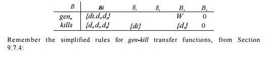
• To take
the meet of transfer functions, take the union of the pen's and the
intersection of the kiWs.
• To
compose transfer functions, take the union of both the pen's and the kill's.
However, as an exception, an expression that is generated by the first
function, not generated by the second, but killed by the second is not in the
gen of the result.
• To take
the closure of a transfer function, retain its gen and replace the kill by 0.
The first
five regions Ri,... , R5 are blocks B1,... , B5, respectively. For 1 < i
< 5, /Ri ( iN[B.] * s *he identity function, and / / j i ( ouT [ Bi ] * s
the transfer function for block Bi:
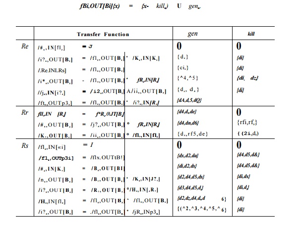
Figure
9.51: Computing transfer functions for the flow graph in Fig. 9.48(a), using
region-based analysis
The rest
of the transfer functions constructed in Step 2 of Algorithm 9.50 are
summarized in Fig. 9.51. Region Re, consisting of regions R2,
R3, and R4,
represents
the loop body and thus does not include the back edge B4 B2. The order of processing these regions will be the only topological order: R2,R3,R4.
First, R2 has no predecessors
within R6; remember that the edge B4
-» B2 goes outside R6. Thus, / R
6 ) T N [ B 2 ] i s t n
e identity function,1 1 and /fl6 ,oUTp32 ] i s the transfer function
for block B2 itself.
The
header of region B3 has
one predecessor within R6:
namely R2. The transfer function
to its entry is simply the transfer function to the exit of B2, / f i 6 , O U T
[ B 2 ] ' which has already been computed.
We compose this function with the transfer function of B3 within its own
region to compute the transfer function to the exit of B3.
Last, for
the transfer function to the entry of R4, we must compute
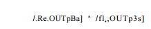
because
both B2 and B3 are predecessors of B4, the header of R4. This transfer function
is composed with the transfer function /i? 4 ,oUT [B 4 ] to get the desired
function /ij6 ,0UT[B4]- Notice, for example, that d3 is not killed in this
transfer function, because the path B2 -» B4 does not redefine variable a.
Now,
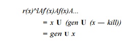
consider loop region R7. It contains only one subregion RQ which represents its
loop body. Since there is only one back edge, B4 —»• B2, to the header of RQ ,
the transfer function representing the execution of the loop body 0 or more
times is just o u T [ s 4 ] :t n e 9
e n s e t is {d4,d^,do}
and the kill set is 0. There are two exits out of region R7, blocks
B3 and B4. Thus, this transfer function is composed with
each of the transfer functions of RQ to get the corresponding transfer
functions of R7. Notice, for instance, how d6 is in the gen set for fn.7,B3 because of paths like B2
->• B4 ->• B2 -» B3, or even
B2 —>
B3 —y B4 B2 —> B3.
Finally,
consider R8, the entire flow graph. Its subregions are Ri, R7, and R5, which we
shall consider in that topological order. As before, the transfer function
/fj8) iN[jBi] is simply the identity function, and the transfer function
/.Rs.OUTpBi] is Just / R I , OUT [ B ! ] , which in turn is fBl.
The
header of R7, which is B2, has only one predecessor, Bi, so the transfer
function to its entry is simply the transfer function out of B1 in region R$.
We compose / ^ 8 ) o u T [ B i ] with the transfer functions to the exits of B3
and B4 within R7 to obtain their corresponding transfer functions within R8.
Lastly, we consider R5. Its header, B5, has two predecessors within R8, namely B3 and B4.
Therefore,
we compute fRs,0VT[B3) A fR8,o1JT[B4] to get /fl 8 ) iN [BB ] - SINCE THE transfer function of block B5 is the identity
function, / R 8 ) OUT [ B6 ] — fR8,lN[B5]-
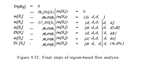
Step 3
computes the actual reaching definitions from the transfer functions. In step
3(a), m[R8] = 0 since there are no reaching definitions at the beginning of the
program. Figure 9.52 shows how step 3(b) computes the rest of the data-flow
values. The step starts with the
subregions of R8. Since the transfer function from the start of R8 to the
start of each of its subregion has been computed, a
single application of the transfer function finds the data-flow value at the
start each subregion. We repeat the steps until we get the data-flow values of
the leaf regions, which are simply the individual basic blocks. Note that the
data-flow values shown in Figure 9.52 are exactly what we would get had we applied
iterative data-flow analysis to the same flow graph, as must be the case, of
course.
6. Handling Nonreducible Flow Graphs
If
nonreducible flow graphs are expected to be common for the programs to be
processed by a compiler or other program-processing software, then we
recom-mend using an iterative rather than a hierarchy-based approach to
data-flow analysis. However, if we need only to be prepared for the occasional
nonre-ducible flow graph, then the following "node-splitting " technique
is adequate.
Construct
regions from natural loops to the extent possible. If the flow graph is
nonreducible, we shall find that the resulting graph of regions has cycles, but
no back edges, so we cannot parse the graph any further. A typical situation is
suggested in Fig. 9.53(a), which has the same structure as the nonreducible
flow graph of Fig. 9.45, but the nodes in Fig. 9.53 may actually be complex
regions, as suggested by the smaller nodes within.
We pick
some region R that has more than one predecessor and is not the header
of the entire flow graph. If i? has k predecessors, make k copies
of the entire flow graph R, and connect each predecessor of i?'s header
to a different copy of R. Remember that only the header of a region
could possibly have a predecessor outside that region. It turns out, although
we shall not prove it, that such node splitting results in a reduction by at
least one in the number of regions, after new back edges are identified and
their regions constructed. The resulting graph may still not be reducible, but
by alternating a splitting phase with a phase where new natural loops are
identified and collapsed to regions, we eventually are left with a single
region; i.e., the flow graph has been reduced.
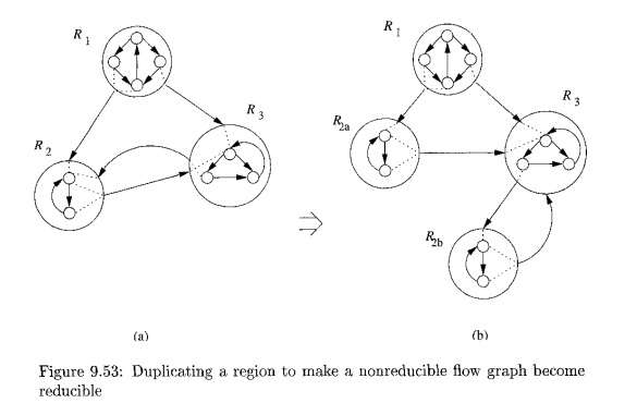
Example 9
. 5 5 : The splitting shown
in Fig. 9.53(b)
has turned the
edge R2b -> R3 into a back edge, since f?3 now dominates R2b- These two regions may thus be combined into one. The resulting three regions — Ri, R2a and the new region — form an acyclic graph,
and therefore may be combined into a single body region.
We thus have reduced the entire flow graph to a single region. In general,
additional splits may be necessary, and in the worst case, the total number of
basic blocks could become exponential in the number of blocks in the original
flow graph. •
We must also think about how the result of the data-flow analysis
on the split flow graph relates to the answer we desire for the original flow
graph. There are two approaches we might consider.
1.
Splitting regions may be beneficial
for the optimization process, and we can simply revise the flow graph to have
copies of certain blocks. Since each duplicated block is entered along only a
subset of the paths that reached the original, the data-flow values at these
duplicated blocks will tend to contain more specific information than was
available at the orig-inal. For instance, fewer definitions may reach each of
the duplicated blocks that reach the original block.
2.
If we wish to retain the original flow
graph, with no splitting, then after analyzing the split flow graph, we look at
each split block B, and its
corresponding set of blocks B1: B2,...
,Bk. We may compute m[B] — m[Bi] A IN[B2
] A • • • A lN[Bf c ], and similarly for the OUT's.
7. Exercises for Section 9.7
Exercise 9 . 7 . 1 : For the flow graph of Fig. 9.10 (see the
exercises for Section 9.1):
i. Find all the possible regions. You may, however, omit from the
list the regions consisting of a single node and no edges.
ii. Give the set of nested regions constructed by
Algorithm 9.52.
Hi. Give a T1-T2 reduction of the flow graph as described in the box on "Where
'Reducible' Comes From" in Section 9.7.2.
Exercise 9 . 7 . 2 : Repeat Exercise 9.7.1 on
the following flow graphs:
a)
Fig. 9.3.
b)
Fig. 8.9.
c)
Your flow graph
from Exercise 8.4.1.
d)
Your flow graph
from Exercise 8.4.2.
Exercise 9 . 7 . 3 : Prove that every natural
loop is a region.
!! Exercise 9 . 7 . 4: Show that a flow graph is reducible if and only it
can be transformed to a single node using:
a) The operations Ti and T2 described in the box in Section 9.7.2.
b) The region definition
introduced in Section 9.7.2.
! Exercise 9 . 7 . 5 : Show that when you apply node splitting to a
nonreducible flow graph, and then perform T1-T2 reduction on
the resulting split graph, you wind up with strictly fewer nodes than you
started with.
! Exercise 9 . 7 . 6 : What happens if you apply node-splitting and T1-T2 reduc-tion alternately, to reduce a complete
directed graph of n nodes?
Related Topics