Chapter: Compilers : Principles, Techniques, & Tools : Machine-Independent Optimizations
Partial-Redundancy Elimination
Partial-Redundancy Elimination
1 The Sources of Redundancy
2 Can All Redundancy Be Eliminated?
3 The Lazy-Code-Motion Problem
4 Anticipation of Expressions
5 The Lazy-Code-Motion Algorithm
6 Exercises for Section 9.5
In this section, we consider in detail how to minimize the number of
expression evaluations. That is, we want to consider all possible execution
sequences in a flow graph, and look at the number of times an expression such
as x + y is evaluated. By moving
around the places where x + y is
evaluated and keeping the result in a temporary variable when necessary, we
often can reduce the number of evaluations of this expression along many of the
execution paths, while not increasing that number along any path. Note that the
number of different places in the flow graph where x + y is evaluated may increase, but that is relatively
unimportant, as long as the number of evaluations
of the expression x + y is reduced.
Applying the code transformation developed here improves the performance
of the resulting code, since, as we shall see, an operation is never applied
unless it absolutely has to be. Every
optimizing compiler implements something like the transformation described here, even if it uses a less "aggressive"
algorithm than the one of this section. However,
there is another motivation for discussing the problem. Finding the right place
or places in the flow graph at which to evaluate each expression requires four
different kinds of data-flow analyses. Thus, the study of
"partial-redundancy elimination," as minimizing the number of
expression evaluations is called, will enhance our understanding of the role
data-flow analysis plays in a compiler.
Redundancy in programs exists in several forms. As discussed in Section
9.1.4, it may exist in the form of common subexpressions, where several
evalua-tions of the expression produce the same value. It may also exist in the
form of a loop-invariant expression that evaluates to the same value in every
iteration of the loop. Redundancy may also be partial, if it is found along
some of the paths, but not necessarily along all paths. Common subexpressions and loop-invariant expressions can
be viewed as special cases of partial redundancy; thus a single
partial-redundancy-elimination algorithm can be devised to eliminate all the
various forms of redundancy.
In the following, we first discuss the different forms of redundancy, in
order to build up our intuition about the problem. We then describe the
generalized redundancy-elimination problem, and finally we present the
algorithm. This algorithm is particularly interesting, because it involves
solving multiple data-flow problems, in both the forward and backward
directions.
1. The Sources of Redundancy
Fi gure 9.30 illustrates the three forms of redundancy: common
subexpressions, loop-invariant expressions, and partially redundant
expressions. The figure shows the code both before and after each optimization.
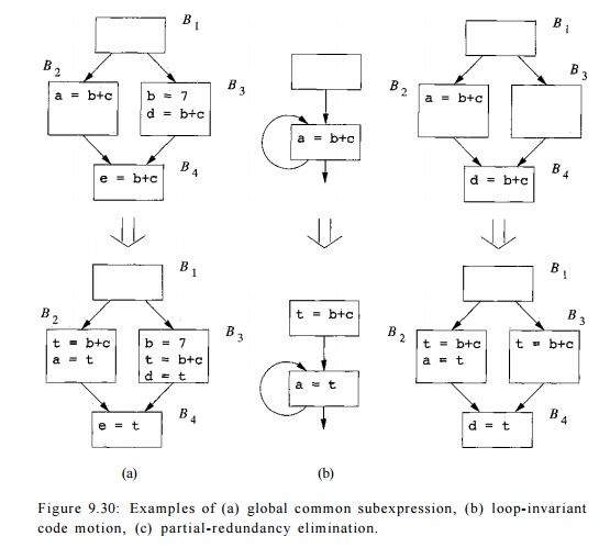
Figure 9.30: Examples of (a) global common subexpression, (b)
loop-invariant code motion, (c) partial-redundancy elimination.
Global Common
Subexpressions
In Fig. 9.30(a), the expression b
+ c computed in block B4 is
redundant; it has already been evaluated by the time the flow of control
reaches B4 regardless of the path tsEken to get there. As we observe in this
example, the value of the expression may be different on different paths. We
can optimize the code by storing the result of the computations of b + c in blocks B2 and B3 in the same temporary variable, say t,
and then assigning the value of t to
the variable e in block B4,
instead of reevaluating the expression. Had there been an assignment to either b or c after the last computation of 6 +
c but before block B4, the
expression in block B4 would not be
redundant.
Formally,
we say that an expression b + c is (fully)
redundant at point p, if it is an available expression, in the sense of
Section 9.2.6, at that point. That is,
the expression b + c has been computed along all paths reaching p, and the
variables b and c were not redefined after the last expression was evaluated.
The latter condition is necessary, because even though the expression b + c is textually
executed before reaching the point p, the value of b + c computed at
Finding "Deep" Common
Subexpressions
Using available-expressions analysis to identify redundant expressions
only works for expressions that are textually identical. For example, an
appli-cation of common-subexpression elimination will recognize that tl in the
code fragment
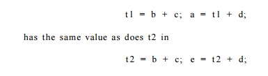
as long as the variables b and
c have not been redefined in between. It does not, however, recognize that a and e are also the same. It is possi-ble to find such "deep"
common subexpressions by re-applying common subexpression elimination until no
new common subexpressions are found on one round. It is also possible to use
the framework of Exercise 9.4.2 to catch deep common subexpressions.
point p would have been different, because the
operands might have changed.
Loop -
Invariant Expressions
Fig.
9.30(b) shows an example of a loop-invariant expression. The expression b + c
is loop invariant assuming neither the variable b nor c is redefined within the
loop. We can optimize the program by replacing all the re-executions in a loop
by a single calculation outside the loop.
We assign the computation to a temporary variable, say t, and then
replace the expression in the loop by t. There is one more point we need to
consider when performing "code motion" optimizations such as this. We
should not execute any instruction that would not have executed without the
optimization. For example, if it is possible to exit the loop without executing
the loop-invariant instruction at all, then we should not move the instruction
out of the loop. There are two reasons.
If the instruction raises an exception, then
executing it may throw an exception that would not have happened in the
original program.
When the loop exits early, the
"optimized" program takes more time than the original program.
To ensure that loop-invariant expressions in
while-loops can be optimized, compilers typically represent the statement
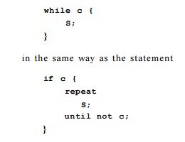
In this
way, loop-invariant expressions can be placed just prior to the repeat-until
construct.
Unlike
common-subexpression elimination, where a redundant expression computation is
simply dropped, loop-invariant-expression elimination requires an expression
from inside the loop to move outside the loop. Thus, this opti-mization is
generally known as "loop-invariant code motion." Loop-invariant code
motion may need to be repeated, because once a variable is determined to to
have a loop-invariant value, expressions using that variable may also become
loop-invariant.
Partially
Redundant Expressions
An
example of a partially redundant expression is shown in Fig. 9.30(c). The
expression b + c in block B4 is redundant on the path B1 -» B2 —> B4, but not on the path B1 ->• B3 ->• B4. We can eliminate the redundancy on
the former path by placing a computation of b
+ c in block B3. All
the results of b + c are written into
a temporary variable t, and the
calculation in block B4 is
replaced with t. Thus, like
loop-invariant code motion, partial-redundancy elimination requires the
placement of new expression computations.
2. Can All Redundancy Be
Eliminated?
Is it possible to eliminate all redundant computations along every path?
The answer is "no," unless we are allowed to change the flow graph by
creating new blocks.
E x a m p l e 9 . 2 8 : In the example shown in Fig. 9.31(a), the
expression of b + c is computed
redundantly in block B4 if the
program follows the execution path Bi B2
-> B4. However, we cannot
simply move the computation of b + c to block B3, because doing so would create an extra
computation of 6 + c when the path B1 -> B3 B5 is taken.
What we would like to do is to insert the computation of b + c only
along the edge from block B3 to block
B4. We can do so by placing the
instruction in a new block, say, BQ, and making the flow of control from B3 go
through B6 before it reaches B4. The transformation is shown in Fig. 9.31(b).
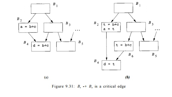
We define a
critical edge of a flow graph to be any edge leading from a node with more than one successor to a node
with more than one predecessor. By introducing new blocks along critical edges,
we can always find a block to accommodate the desired expression placement. For instance, the edge from B3 to B4
in Fig. 9.31(a) is critical, because B3 has two successors, and B4 has two predecessors.
Adding blocks may not be sufficient to allow the elimination of all
redundant computations. As shown in Example 9.29, we may need to duplicate code
so as to isolate the path where redundancy is found.
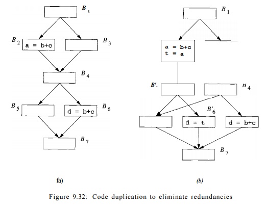
Example 9 . 2 9 : In the example shown in Figure 9.32(a), the expression
of b+c is computed redundantly along the path B1 -+ B2 -+ B4 —> BQ . We
would like to remove the redundant computation of b + c from block BQ in this
path and compute the expression only along the path B1 -+ B3 -+ B4 -+ BQ.
However, there is no single program point or edge in the source program that
corresponds uniquely to the latter path. To create such a program point, we can
duplicate the pair of blocks B4 and BQ , with one pair reached through B2 and
the other reached through B3: as shown in Figure 9.32(b). The result of b + c
is saved in variable t in block B2, and moved to variable d in B'Q, the copy of
BQ reached from B2. •
Since the number of paths is exponential in the number of conditional
branches in the program, eliminating all redundant expressions can greatly
increase the size of the optimized code. We therefore restrict our discussion
of redundancy-elimination techniques to those that may introduce additional
blocks but that do not duplicate portions of the control flow graph.
3. The Lazy-Code-Motion Problem
It is desirable for programs optimized with a partial-redundancy-elimination
algorithm to have the following properties:
All redundant computations of
expressions that can be eliminated without code duplication are eliminated.
The optimized program does not
perform any computation that is not in the original program execution.
3. Expressions are computed at the latest possible time.
The last property is important because the values of expressions found
to be redundant are usually held in registers until they are used. Computing a
value as late as possible minimizes its lifetime — the duration between the
time the value is defined and the time it is last used, which in turn minimizes
its usage of a register. We refer to the optimization of eliminating partial
redundancy with the goal of delaying the computations as much as possible as lazy code motion.
To build up our intuition of the problem, we first discuss how to reason
about partial redundancy of a single expression along a single path. For
convenience, we assume for the rest of the discussion that every statement is a
basic block of its own.
Full Redundancy
An expression e in block B is
redundant if along all paths reaching B,
e has been evaluated and the operands of e have not been redefined
subsequently. Let S be the set of
blocks, each containing expression e, that renders e in B redundant. The set of edges leaving the blocks in S must necessarily form a cutset, which if removed, disconnects
block B from the entry of the
program. Moreover, no operands of e
are redefined along the paths that lead from the blocks in S to B.
Partial Redundancy
If an expression e in block B
is only partially redundant, the lazy-code-motion algorithm attempts to render
e fully redundant in B by placing
additional copies of the expressions in the flow graph. If the attempt is
successful, the optimized flow graph will also have a set of basic blocks 5, each containing expression e, and whose outgoing edges are a cutset
between the entry and B. Like the
fully redundant case, no operands of e are redefined along the paths that lead
from the blocks in S to B.
4. Anticipation of Expressions
There is an additional constraint imposed on inserted expressions to
ensure that no extra operations are executed. Copies of an expression must be
placed only at program points where the expression is anticipated. We say that an expression b + c is anticipated at point p if all paths leading from the point p eventually compute the value of the
expression b + c from the values of b and c that are available at that
point.
Let us
now examine what it takes to eliminate partial redundancy along an acyclic
path Bi -+ B2
-»...-» Bn. Suppose
expression e is evaluated
only in blocks B\ and Bn, and
that the operands of e are not redefined in blocks along the path. There are
incoming edges that join the path and there are outgoing edges that exit the
path. We see that e is not anticipated at the entry of block Bi if and only if
there exists an outgoing edge leaving block Bj, i < j < n, that leads to
an execution path that does not use the value of e. Thus, anticipation limits
how early an expression can be inserted.
We can
create a cutset that includes the edge B^i -+ Bi and that renders e redundant
in Bn if e is either available or anticipated at the entry of Bi. If e is anticipated but not available at the
entry of Bi, we must place a copy of the expression e along the incoming edge.
We have a
choice of where to place the copies of the expression, since there are usually
several cutsets in the flow graph that satisfy all the requirements. In the
above, computation is introduced along the incoming edges to the path of
interest and so the expression is computed as close to the use as possible,
without introducing redundancy. Note that these introduced operations may
themselves be partially redundant with other instances of the same expression
in the program. Such partial redundancy may be eliminated by moving these
computations further up.
In
summary, anticipation of expressions limits how early an expression can be
placed; you cannot place an expression so early that it is not anticipated
where you place it. The earlier an expression is placed, the more redundancy
can be removed, and among all solutions that eliminate the same redundancies,
the one that computes the expressions the latest minimizes the lifetimes of the
registers holding the values of the expressions involved.
5. The Lazy-Code-Motion Algorithm
This discussion thus motivates a four-step algorithm. The first step
uses an-ticipation to determine where expressions can be placed; the second
step finds the earliest cutset, among
those that eliminate as many redundant operations as possible without
duplicating code and without introducing any unwanted computations. This step
places the computations at program points where the values of their results are
first anticipated. The third step then pushes the cutset down to the point
where any further delay would alter the semantics of the program or introduce
redundancy. The fourth and final step is a simple pass to clean up the code by
removing assignments to temporary variables that are used only once. Each step
is accomplished with a data-flow pass: the first and fourth are backward-flow
problems, the second and third are forward-flow problems.
Algorithm Overview
Find all the expressions
anticipated at each program point using a back-ward data-flow pass.
The second step places the
computation where the values of the expres-sions are first anticipated along
some path. After we have placed copies of an expression where the expression is
first anticipated, the expression would be available
at program point p if it has been
anticipated along all paths reaching p.
Availability can be solved using a forward data-flow pass. If we wish to place
the expressions at the earliest possible posi-tions, we can simply find those
program points where the expressions are anticipated but are not available.
Executing an expression as soon
as it is anticipated may produce a value long before it is used. An expression
is postponable at a program point if
the expression has been anticipated and has yet to be used along any path
reaching the program point. Postponable expressions are found using a forward
data-flow pass. We place expressions at those program points where they can no longer
be postponed.
A simple, final backward data-flow pass is used to eliminate assignments
to temporary variables that are used only once in the program.
Preprocessing Steps
We now present the full lazy-code-motion algorithm. To keep the
algorithm simple, we assume that initially every statement is in a basic block
of its own, and we only introduce new computations of expressions at the
beginnings of blocks. To ensure that this simplification does not reduce the
effectiveness of the technique, we insert a new block between the source and
the destination of an edge if the destination has more than one predecessor.
Doing so obviously also takes care of all critical edges in the program.
We abstract the semantics of each block B with two sets: e-uses is the set of expressions computed in
B and e-kills is the set of expressions
killed, that is, the set of expressions any of whose operands are defined in B.
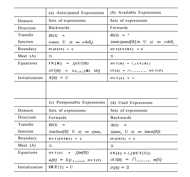
Example 9.30 will be used throughout the discussion of the four data-flow
analyses whose definitions are summarized in Fig. 9.34.
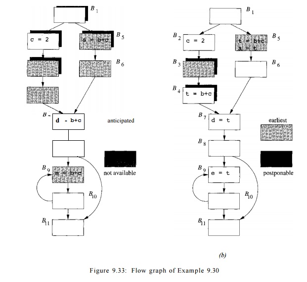
Example 9 . 3 0 : In the flow graph in Fig. 9.33(a), the expression b + c appears three
times. Because the block B9 is part of a loop, the expression may be computed
many times. The computation in block BQ is not only loop invariant; it is also
a redundant expression, since its value already has been used in block Bj. For
this example, we need to compute b+c only twice, once in block B5 and once
along the path after B2 and before B7.
The lazy code motion algorithm will place the expression computations at the
beginning of blocks B4 and B5.
Anticipated Expressions
Recall that an expression b + c
is anticipated at a program point p
if all paths leading from point p
eventually compute the value of the expression b + c from the values of b
and c that are available at that point.
In Fig. 9.33(a), all the blocks anticipating b + c on entry are shown as lightly shaded boxes. The expression b + c is anticipated in blocks £3, B4, . B 5 , B6, BJ, and BQ. It is not anticipated on entry to block B2, because
the value of c is recomputed within the block, and therefore the value of b + c that would be computed at the
beginning of B2 is not used along any path. The expression b+c is not anticipated on entry to B1, because it is unnecessary along the branch from B1 to B2 (although it would be used along the path B1 —> B5 -> B6). Similarly, the expression is not
anticipated at the beginning of B8, because of the branch from B8 to Bn. The anticipation of an
expression may oscillate along a path, as illustrated by £7 —> Bg —> BQ.
The data-flow equations for the anticipated-expressions problem are
shown in Fig 9.34(a). The analysis is a backward pass. An anticipated
expression at the exit of a block B
is an anticipated expression on entry only if it is not in the e-kills set. Also a block B generates as new uses the set of ejuses expressions. At the exit of the program, none of the expressions are
anticipated. Since we are interested in finding expressions that are
anticipated along every subsequent
path, the meet operator is set intersection. Consequently, the interior
points must be initialized to the universal set U, as was discussed for the available-expressions problem in
Section 9.2.6.
Available Expressions
At the end of this second step, copies of an expression will be placed
at program points where the expression is first anticipated. If that is the
case, an expression will be available
at program point p if it is
anticipated along all paths reaching p. This
problem is similar to available-expressions described in Section 9.2.6. The transfer function used here is
slightly different though. An expression is available on exit from a block if
it is
Completing the Square
Anticipated expressions (also called "very busy expressions"
elsewhere) is a type of data-flow analysis we have not seen previously. While
we have seen backwards-flowing frameworks such as live-variable analysis (Sect.
9.2.5), and we have seen frameworks where the meet is intersection such as
avail-able expressions (Sect. 9.2.6), this is the first example of a useful
analysis that has both properties. Almost all analyses we use can be placed in
one of four groups, depending on whether they flow forwards or backwards, and
depending on whether they use union or intersection for the meet. Notice also
that the union analyses always involve asking about whether there exists a path
along which something is true, while the intersection analyses ask whether
something is true along all paths.
1. Either
(a) Available, or
(b) In the set of
anticipated expressions upon entry
(i.e., it could be
made available if we chose to compute it here), and
2. Not killed in the block.
The data-flow equations for available expressions are shown in Fig
9.34(b). To avoid confusing the meaning of IN, we refer to the result of an
earlier analysis by appending "[JBj.m" to the name of the earlier
analysis.
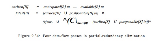
With the earliest placement strategy, the set of expressions placed at
block B, i.e., earliest[B], is defined as the set of anticipated expressions
that are not yet available. That is,
earliest[B] — anticipated[B].in —
available[B].in.
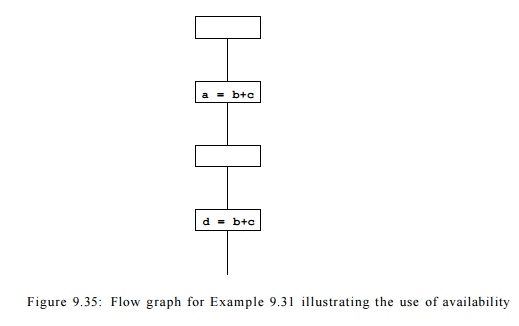
Example 9 . 3 1 : The expression
b + c in the flow graph in Figure 9.35 is not anticipated at the entry of block
B3 but is anticipated at the entry of
block B4. It is, however, not necessary to compute the expression 6 + c in
block B4, because the expression is already available due to block B2.
Example 9 . 3 2 : Shown with dark shadows in Fig. 9.33(a) are the blocks
for which expression b + c is
not available; they
are Bi,B2,B3, and B5. The early-placement positions are
represented by the lightly shaded boxes with dark shadows, and are thus blocks
B3 and B5 . Note, for instance, that b + c is considered available on entry to
B4, because there is a path B1 -» B2 -> B3 —»• B4 along which b + c is
anticipated at least once — at B3 in this case — and since the beginning of B3,
neither b nor c was recomputed.
Postponable Expressions
The third step postpones the computation of expressions as much as
possible while preserving the original program semantics and minimizing
redundancy. Example 9.33 illustrates the importance of this step.
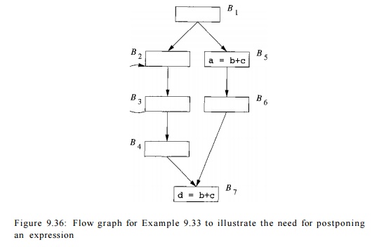
Example 9 . 3 3 : In the flow graph shown in Figure 9.36, the expression b
+ c is computed twice along the
path Bi -+ B5 -» BQ -» B7. The
expression b + c is anticipated even
at the beginning of block B1. If we
compute the expression as soon as it is anticipated, we would have computed the
expression b + c in B1. The result would have to be saved
from the beginning, through the execution of the loop comprising blocks B2 and £3, until it is used in block B7.
Instead we can delay the computation of expression b + c until the beginning of B5 and until the flow of control is about to transition from B4 to Bq. •
Formally, an expression x + y
is postponable to a program point p
if an early placement of x + y is
encountered along every path from the entry node to p, and there is no subsequent use of x + y after the last such placement.
Example 9 . 3 4 : Let us again consider expression b + c in Fig. 9.33. The two earliest points for b + c are B3 and B5; note that these are the two blocks that are both lightly and darkly
shaded in Fig. 9.33(a), indicating that b
+ c is both anticipated and not available for these blocks, and
only these blocks. We cannot postpone b +
c from B5 to BQ , because b + c is used in B5.
We can postpone it from B3
to B4, however.
But we
cannot postpone b + c from B4 to B7.
The reason is that, although b + c is not used in B4, placing its computation
at B7 instead would lead to a
redundant
computation of b + c along the path B§
-» BQ -» B7. As we shall see, B4
is one of the latest places we can compute b + c.
The
data-flow equations for the postponable-expressions problem are shown in Fig
9.34(c). The analysis is a
forward pass. We cannot
"postpone" an expression to
the entry of the program, so OUT [ ENTRY ] = 0. An expression is postponable to
the exit of block B if it is not used in the block, and either it is postponable to the
entry of B or it is in
earliest[B]. An expression is not postponable to the entry of a block unless
all its predecessors include the expression in their postponable sets at their
exits. Thus, the meet operator is set intersection, and the interior points
must be initialized to the top element of the semilattice — the universal set.
Roughly
speaking, an expression is placed at the frontier
where an expression transitions from being postponable to not being
postponable. More specifically, an expression e may be placed at the beginning
of a block B only if the expres-sion
is in B's earliest or postponable set upon entry. In addition,
B is in the postponement frontier of
e if one of the following holds:
1. e is
not in postponable[B].out. In other words, e is in ejuses-
Expression
e can be placed at the front of block B
in either of the above scenarios because of the new blocks introduced by the
preprocessing step in the algorithm.
E x a m p l e 9 . 3 5 : Fig.
9.33(b) shows the result of the analysis. The light-shaded boxes represent the blocks whose earliest set includes b + c.
The dark shadows indicate those that include b + c in their postponable
set. The latest placements of the expressions are thus the entries of blocks B4 and B5, since
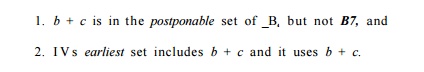
1. b + c
is in the postponable set of _B4 but
not B7, and
2. I V s
earliest set includes b + c and it uses b + c.
The
expression is stored into the temporary variable t in blocks B4 and B5, and t
is used in place of b + c everywhere else, as shown in the figure.
U s e d Expressions
Finally,
a backward pass is used to determine if the temporary variables in-troduced are
used beyond the block they are in. We say that an expression is used at point p if there exists a path leading from p that uses the expression before
the value is reevaluated. This analysis is essentially liveness analysis (for
expressions, rather than for variables).
The data-flow equations for
the used expressions
problem are shown
in Fig 9.34(d). The analysis is a
backward pass. A used expression at the
exit of a block B is a used expression
on entry only if it is not in the latest set.
A block
generates, as new uses, the set of expressions in ejuse^ . At the exit of the
program, none of the expressions are used. Since we are interested in finding
expressions that are used by any subsequent path, the meet operator is set
union. Thus, the interior points must be initialized with the top element of
the semilattice — the empty set.
Putting it
All Together
All the
steps of the algorithm are summarized in Algorithm 9.36.
Algorithm 9.36 :
Lazy code motion.
INPUT: A
flow graph for
which ejuses and
eJtillB have been
computed for each block B.
OUTPUT: A modified flow graph satisfying
the four lazy code motion conditions in Section 9.5.3.
METHOD:
Insert an empty block along all edges entering
a block with more than one predecessor.
2. Find
anticipated[B].in for all blocks B,
as defined in Fig. 9.34(a).
3. Find
available[B].in for all blocks B as defined in Fig. 9.34(b).
4. Compute the earliest placements for all
blocks B:
earliest[B] = anticipated[B].in - available[B].in
5. Find postponable[B).in for all blocks B as
defined in Fig. 9.34(c).
6.
Compute the latest placements for all blocks B:
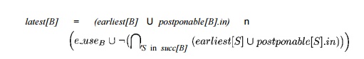
Note that
-i denotes complementation with respect to the set of all ex-pressions computed
by the program.
7. Find used[B].out for all blocks B,
as defined in Fig. 9.34(d).
8. For
each expression, say x+y, computed by
the program, do the following:
(a) Create a new temporary, say t, for x + y.
(b) For
all blocks B such that x + y is in latest[B] n used[B].out, add
t = x+y
at the beginning of B.
For all blocks B
such that x + y is in
ejuses H (->latest[B] U used.out[B])
replace
every original x + y by t.
•
S u m m a r y
Partial-redundancy
elimination finds many different forms of redundant opera-tions in one unified
algorithm. This algorithm illustrates how multiple data-flow problems can be
used to find optimal expression placement.
The placement constraints are provided by the
anticipated-expressions analysis, which is a backwards data-flow analysis with a set-intersection meet operator,
as it determines if expressions are used subsequent
to each program point on all paths.
The earliest
placement of an expression is given by program points where the expression is
anticipated but is not available. Available expressions are found with a forwards data-flow analysis with a
set-intersection meet operator that computes if an expression has been
anticipated before each program point
along all paths.
The latest placement of an expression is given by
program points where an expression can no longer be postponed. Expressions are
postponable at a program point if for all
paths reaching the program point, no
use of the expression has been encountered. Postponable expressions are found
with a forwards data-flow analysis with a
set-intersection meet operator.
Temporary assignments are eliminated unless they
are used by some path subsequently. We find used expressions
with a backwards data-flow anal-ysis,
this time with a set-union meet operator.
6. Exercises for Section 9.5
Exercise 9.5.1: For the flow graph
in Fig. 9.37:
a) Compute anticipated
for the beginning and end of each block.
b) Compute available
for the beginning and end of each block.
Compute earliest for each block.
Compute postponable
for the beginning and end of each block.
e) Compute used
for the beginning and end of each block.
f) Compute
latest for each block.
Introduce temporary variable t; show where it is computed and where it is used.
Exercise 9.5.2: Repeat Exercise 9.5.1 for the
flow graph of Fig. 9.10 (see the exercises to Section 9.1). You
may limit your analysis to the expressions a
+ 6, c — a, and b * d.
Exercise 9.5.3: The concepts discussed in this
section can also be applied to eliminate partially dead code. A
definition of a variable is partially
dead if the variable is live on some paths and not others. We can optimize
the program execution by only performing the definition along paths where the
variable is live. Unlike partial-redundancy elimination, where expressions are
moved before the original, the new definitions are placed after the original.
Develop an algorithm to move partially dead code, so expressions are evaluated
only where they will eventually be used.
Related Topics