Loops in Flow Graphs

Loops in Flow Graphs

1 Dominators

2 Depth-First Ordering

3 Edges in a Depth-First Spanning Tree

4 Back Edges and Reducibility

5 Depth of a Flow Graph

6 Natural Loops

7 Speed of Convergence of Iterative Data-Flow Algorithms

8 Exercises for Section 9.6

In our discussion so far, loops have not been handled differently; they have been treated just like any other kind of control flow. However, loops are important because programs spend most of their time executing them, and optimizations

that improve the performance of loops can have a significant impact. Thus, it is essential that we identify loops and treat them specially.

Loops also affect the running time of program analyses. If a program does not contain any loops, we can obtain the answers to data-flow problems by making just one pass through the program. For example, a forward data-flow problem can be solved by visiting all the nodes once, in topological order.

In this section, we introduce the following concepts: dominators, depth-first ordering, back edges, graph depth, and reducibility. Each of these is needed for our subsequent discussions on finding loops and the speed of convergence of iterative data-flow analysis.

1. Dominators

We say node d of a flow graph dominates node n, written d dom n, if every path from the entry node of the flow graph to n goes through d. Note that under this definition, every node dominates itself.

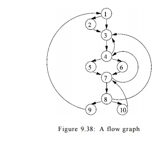
E x a m p l e 9 . 3 7 : Consider the flow graph of Fig. 9.38, with entry node 1. The entry node dominates every node (this statement is true for every flow graph). Node 2 dominates only itself, since control can reach any other node along a path that begins with 1 -> 3. Node 3 dominates all but 1 and 2. Node 4 dominates all but 1, 2 and 3, since all paths from 1 must begin with l - > - 2 - > - 3 - > - 4 o r 1 3 4. Nodes 5 and 6 dominate only themselves, since flow of control can skip around either by going through the other. Finally, 7 dominates 7, 8, 9, and 10; 8 dominates 8, 9, and 10; 9 and 10 dominate only themselves.

A useful way of presenting dominator information is in a tree, called the dominator tree, in which the entry node is the root, and each node d dominates only its descendants in the tree. For example, Fig. 9.39 shows the dominator tree for the flow graph of Fig. 9.38.

The existence of dominator trees follows from a property of dominators: each node n has a unique immediate dominator m that is the last dominator of n on any path from the entry node to n. In terms of the dom relation, the immediate dominator m has that property that if d  ^  n  and d dom  n,  then d dom  m.   

We shall give a simple algorithm for computing the dominators of every node n in a flow graph, based on the principle that if pi,p2, • • • ,Pk are all the predecessors of n, and d ^ n, then d dom n if and only if d dom pi for each i.

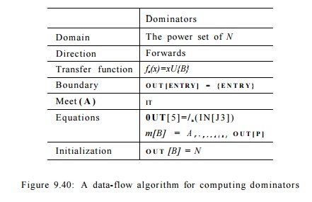
This problem can be formulated as a forward data-flow analysis.  The data-flow values are sets of basic blocks.  A node's set of dominators, other than itself, is the intersection of the dominators of all its predecessors; thus the meet operator is set intersection.  The transfer function for block B simply adds B itself to the set of input nodes.  The boundary condition is that the E N T R Y  node dominates itself.  Finally, the initialization of the interior nodes is the universal set, that is, the set of all nodes.   

Algorithm 9 . 3 8 : Finding dominators.  

INPUT: A flow graph G with set of nodes N, set of edges E and entry node ENTRY .    

OUTPUT: D(n), the set of nodes that dominate node n, for all nodes n in N.

METHOD: Find the solution to the data-flow problem whose parameters are shown in Fig. 9.40. The basic blocks are the nodes. D(n) = OUT [n] for all n in

Finding dominators using this data-flow algorithm is efficient. Nodes in the graph need to be visited only a few times, as we shall see in Section 9.6.7.

Example 9 . 3 9 :  Let  us return to the flow graph of Fig.  9.38,  and suppose the for-loop of lines (4) through (6) in Fig. 9.23 visits the nodes in numerical order.  Let D(n) be the set of nodes in  OUT[n]. Since  1 is the entry node, D(l)  was assigned {1}  at line  (1).  Node 2 has only  1 for a predecessor,  so 

Properties of the dom Relation

A key observation about dominators is that if we take any acyclic path from the entry to node n, then all the dominators of n appear along this path, and moreover, they must appear in the same order along any such path. To see why, suppose there were one acyclic path Pi to n along which dominators a and b appeared in that order and another path P₂ to n, along which b preceded a. Then we could follow Pi to a and P₂ to n, thereby avoiding b altogether. Thus, b would not really dominate a.

This reasoning allows us to prove that dom is transitive: if a dom b and b dom c, then a dom c. Also, dom is antisymmetric: it is never possible that both a dom b and b dom a hold, if a / b. Moreover, if a and b are two dominators of n, then either a dom 6 or & dom a must hold. Finally, it follows that each node n except the entry must have a unique immediate dominator — the dominator that appears closest to n along any acyclic path from the entry to n.

D(2) = { 2 } U D ( 1 ) . Thus, D{2) is set to {1, 2}. Then node 3, with predecessors 1, 2, 4, and 8, is considered. Since all the interior nodes are initialized with the universal  set  N,

£>(3) = {3} U ({1} n {1,2} n { 1 , 2 , . . . , 10} n { 1 , 2 , . . . , 10}) = {1,3}

The remaining calculations are shown in Fig. 9.41. Since these values do not change in the second iteration through the outer loop of lines (3) through (6) in Fig. 9.23(a), they are the final answers to the dominator problem. •

D(4) = {4} U (D(3) n D(7)) = {4} U ({1,3} n { 1 , 2 , . . . , 10}) = {1,3,4}

D(5) = {5} U P ( 4 ) = {5} U {1,3,4} = {1,3,4,5}

D(6) = {6} U 0 ( 4 ) = {6} U {1,3,4} = {1,3,4,6}

D{7) = {7} U (U(5) n D(6) n £>(10))

= {7} U ({1,3,4,5} n {1,3,4,6} n { 1 , 2 , . . . , 10}) = {1,3,4,7}

D(S) = {8} U D{7) = {8} U {1,3,4,7} = {1,3,4,7,8}

D(9) = {9} U D(8) = {9} U {1,3,4,7,8} = {1,3,4,7,8,9}

D(10) = {10} U £>(8) = {10} U {1,3,4,7,8} = {1,3,4,7,8,10}

Figure 9.41:  Completion of the dominator calculation for Example 9.39

2. Depth-First Ordering

As introduced in Section 2.3.4, a depth-first search of a graph visits all the nodes in the graph once, by starting at the entry node and visiting the nodes as far away from the entry node as quickly as possible. The route of the search in a depth-first search forms a depth-first spanning tree (DFST). Recall from Section 2.3.4 that a preorder traversal visits a node before visiting any of its children, which it then visits recursively in left-to-right order. Also, a postorder traversal visits a node's children, recursively in left-to-right order, before visiting the node itself.

There is one more variant ordering that is important for flow-graph analysis: a depth-first ordering is the reverse of a postorder traversal. That is, in a depth-first ordering, we visit a node, then traverse its rightmost child, the child to its left, and so on. However, before we build the tree for the flow graph, we have choices as to which successor of a node becomes the rightmost child in the tree, which node becomes the next child, and so on. Before we give the algorithm for depth-first ordering, let us consider an example.

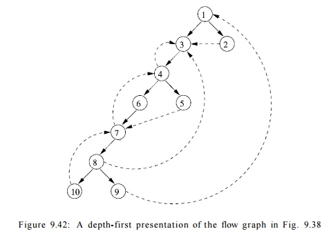
E x a m p l e 9 . 4 0 : One possible depth-first presentation of the flow graph in Fig. 9.38 is illustrated in Fig. 9.42. Solid edges form the tree; dashed edges are the other edges of the flow graph. A depth-first traversal of the tree is given by: 1 -> 3 ->• 4 -» 6 -> 7 -»• 8 ->• 10, then back to 8, then to 9. We go back to 8 once more, retreating to 7, 6, and 4, and then forward to 5. We retreat from 5 back to 4, then back to 3 and 1. From 1 we go to 2, then retreat from 2, back to 1, and we have traversed the entire tree.

The preorder sequence for the traversal is thus

1,3,4,6,7,8,10,9,5,2 .

The postorder sequence for the traversal of the tree in Fig. 9.42 is

1 0 , 9 , 8 , 7 , 6 , 5 , 4 , 3 , 2 , 1 .

The depth-first ordering, which is the reverse of the postorder sequence, is

1,2,3,4,5,6,7,8,9,10 .

•

We now give an algorithm that finds a depth-first spanning tree and a depth-first ordering of a graph. It is this algorithm that finds the DFST in Fig. 9.42 from Fig. 9.38.

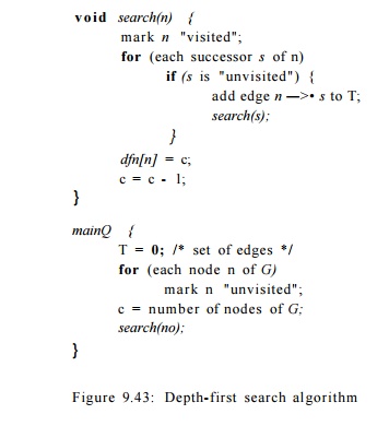
Algorithm 9 . 4 1 :  Depth-first spanning tree and depth-first ordering.

INPUT : A flow graph G.

OUTPUT : A DFST T of G and an ordering of the nodes of G.

METHOD : We use the recursive procedure search(n) of Fig. 9.43. The algo- rithm initializes  all nodes of G to  "unvisited," then calls search(no), where no is the entry.  When it calls search(n), it first marks n "visited" to avoid adding n to the tree twice. It uses c to count from the number of nodes of G down to 1, assigning depth-first numbers dfn[n] to nodes n as we go. The set of edges T forms the depth-first spanning tree for G.

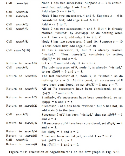
Example 9 . 4 2 : For the flow graph in Fig. 9.42, Algorithm 9.41 sets c to 10 and begins the search by calling search(l). The rest of the execution sequence is shown in Fig. 9.44. •      

3. Edges in a Depth-First Spanning Tree

When we construct a DFST for a flow graph, the edges of the flow graph fall into three categories.

1. There are edges, called advancing edges, that go from a node m to a proper descendant of m in the tree. All edges in the DFST itself are advancing edges. There are no other advancing edges in Fig. 9.42, but, for example,

if 4 —>• 8 were an edge, it would be in this category.

2. There are edges that go from a node m to an ancestor of m in the tree (possibly to m itself). These edges we shall term retreating edges. For example, 4 - > 3 , 7 - > 4 , 1 0 - » 7 and 9 ->• 1 are the retreating edges in Fig. 9.42.

3. There are edges m —> n such that neither m nor n is an ancestor of the other in the DFST . Edges 2 - > 3 and 5 -> 7 are the only such examples in Fig. 9.42. We call these edges cross edges. An important property of cross edges is that if we draw the DFST so children of a node are drawn

1 from left to right in the order in which they were added to the tree, then all cross edges travel from right to left.

It should be noted that m ->• n is a retreating edge if and only if dfn[m] > dfn[n]. To see why, note that if m is a descendant of n in the DFST, then search(m)  terminates  before  search(n),  so dfn[m]  > dfn[n]. Conversely,  if dfn[m]  >  dfn[n],  then  search(m)  terminates before  search(n),  or m = n.  But search(n) must have begun before search(m) if there is an edge m —> n, or else the fact that n is a successor of m would have made n a descendant of m in the DFST . Thus the time search(m) is active is a subinterval of the time search(n) is active, from which it follows that n is an ancestor of m in the DFST .

Back Edges and Reducibility

A  back edge is an edge a  ->  b whose head b dominates its tail a.  For any flow graph, every back edge is retreating, but not every retreating edge is a back edge. A flow graph is said to be  reducible if all its retreating edges in any depth-first spanning tree are also back edges. In other words, if a graph is reducible, then all the DFST's have the same set of retreating edges, and  

Why Are Back Edges Retreating Edges?

Suppose a —> b is a back edge; i.e., its head dominates its tail. The sequence of calls of the function search in Fig. 9.43 that lead to node a must be a path in the flow graph. This path must, of course, include any dominator of a. It follows that a call to search(b) must be open when search(a) is called. Therefore b is already in the tree when a is added to the tree, and o is added as a descendant of b. Therefore, a b must be a retreating edge. 

those are exactly the back edges in the graph. If the graph is nonreducible (not reducible), however, all the back edges are retreating edges in any DFST, but each DFST may have additional retreating edges that are not back edges. These retreating edges may be different from one DFST to another. Thus, if we remove all the back edges of a flow graph and the remaining graph is cyclic, then the graph is nonreducible, and conversely.

Flow graphs that occur in practice are almost always reducible. Exclusive use of structured flow-of-control statements such as if-then-else, while-do, con-tinue, and break statements produces programs whose flow graphs are always reducible. Even programs written using goto statements often turn out to be

reducible, as the programmer logically thinks in terms of loops and branches.

E x a m p l e 9 . 4 3 :  The flow graph of Fig. 9.38 is reducible.  The retreating edges

in the graph are all back edges; that is, their heads dominate their respective tails.  

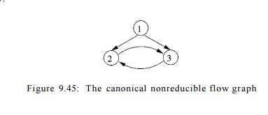
E x a m p l e 9 . 4 4 : Consider the flow graph of Fig. 9.45, whose initial node is 1. Node 1 dominates nodes 2 and 3, but 2 does not dominate 3, nor vice-versa. Thus, this flow graph has no back edges, since no head of any edge dominates its tail. There are two possible depth-first spanning trees, depending on whether we choose to call search(2) or search(3) first, from search(l). In the first case, edge 3 -» 2 is a retreating edge but not a back edge; in the second case, 2 3 is the retreating-but-not-back edge. Intuitively, the reason this flow graph is not reducible is that the cycle 2-3 can be entered at two different places, nodes 2 and 3.

5. Depth of a Flow Graph

Given a depth-first spanning tree for the graph, the depth is the largest number of retreating edges on any cycle-free path. We can prove the depth is never greater than what one would intuitively call the depth of loop nesting in the flow graph. If a flow graph is reducible, we may replace "retreating" by "back" in the definition of "depth," since the retreating edges in any DFST are exactly the back edges. The notion of depth then becomes independent of the DFST actually chosen, and we may truly speak of the "depth of a flow graph," rather than the depth of a flow graph in connection with one of its depth-first spanning trees.

with three retreating edges, but no cycle-free path with four or more retreating edges. It is a coincidence that the "deepest" path here has only retreating edges; in general we may have a mixture of retreating, advancing, and cross edges in a deepest path. •

6. Natural Loops

Loops can be specified in a source program in many different ways: they can be written as for-loops, while-loops, or repeat-loops; they can even be defined using labels and goto statements. From a program-analysis point of view, it does not matter how the loops appear in the source code. What matters is whether they have the properties that enable easy optimization. In particular, we care about whether a loop has a single-entry node; if it does, compiler analyses can assume certain initial conditions to hold at the beginning of each iteration through the loop. This opportunity motivates the need for the definition of a "natural loop."

            natural loop is defined by two essential properties.

            It must have a single-entry node, called the header. This entry node dominates all nodes in the loop, or it would not be the sole entry to the loop.

            There must be a back edge that enters the loop header. Otherwise, it is not possible for the flow of control to return to the header directly from the "loop"; i.e., there really is no loop.

Given a back edge n ->• d, we define the natural loop of the edge to be d plus the set of nodes that can reach n without going through d. Node d is the header of the loop.

Algorithm 9.46 :  Constructing the natural loop of a back edge.

INPUT : A flow graph G and a back edge n -> d.

OUTPUT : The set loop consisting of all nodes in the natural loop of n -> d.

METHOD : Let loop be {n, d}. Mark d as "visited," so that the search does not reach beyond d. Perform a depth-first search on the reverse control-flow graph starting with node n. Insert all the nodes visited in this search into loop. This procedure finds all the nodes that reach n without going through d.

Example 9 . 4 7 :  In Fig.  9.38, there are five back edges, those whose heads dominate their tails: 10 7, 7 -+ 4, 4 -» 3, 8 ->• 3 and 9 1. Note that these are exactly the edges that one would think of as forming loops in the flow graph.

Back edge 10 -> 7 has natural loop {7,8,10}, since 8 and 10 are the only nodes that can reach 10 without going through 7. Back edge 7 -> 4 has a natural loop consisting of {4,5,6,7,8,10} and therefore contains the loop of 10 —>• 7. We thus assume the latter is an inner loop contained inside the former.

The natural loops of back edges 4 3 and 8 ->• 3 have the same header, node 3, and they also happen to have the same set of nodes: {3,4,5,6,7,8,10} . We shall therefore combine these two loops as one. This loop contains the two smaller loops discovered earlier.

Finally, the edge 9 -> 1 has as its natural loop the entire flow graph, and therefore is the outermost loop. In this example, the four loops are nested within one another. It is typical, however, to have two loops, neither of which is a subset of the other. •

In reducible flow graphs, since all retreating edges are back edges, we can associate a natural loop with each retreating edge. That statement does not hold for nonreducible graphs. For instance, the nonreducible flow graph in Fig. 9.45 has a cycle consisting of nodes 2 and 3. Neither of the edges in the cycle is a back edge, so this cycle does not fit the definition of a natural loop. We do not identify the cycle as a natural loop, and it is not optimized as such. This situation is acceptable, because our loop analyses can be made simpler by assuming that all loops have single-entry nodes, and nonreducible programs are rare in practice anyway.

By considering only natural loops as "loops," we have the useful property that unless two loops have the same header, they are either disjoint or one is nested within the other. Thus, we have a natural notion of innermost loops: loops that contain no other loops.

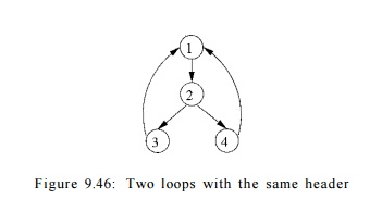
When two natural loops have the same header, as in Fig. 9.46, it is hard to tell which is the inner loop. Thus, we shall assume that when two natural loops have the same header, and neither is properly contained within the other, they are combined and treated as a single loop.

E x a m p l e 9 . 4 8 : The natural loops of the back edges 3 -»• 1 and 4 -> 1 in Fig. 9.46 are {1,2,3} and {1,2,4}, respectively. We shall combine them into a single loop, {1,2,3,4} .

However,  were there another back edge 2  -> 1  in Fig.  9.46,  its natural loop would be {1, 2}, a third loop with header 1. This set of nodes is properly contained within {1, 2,3,4}, so it would not be combined with the other natural loops, but rather treated as an inner loop, nested within. 

7. Speed of Convergence of Iterative Data-Flow Algorithms

We are now ready to discuss the speed of convergence of iterative algorithms. As discussed in Section 9.3.3, the maximum number of iterations the algorithm may take is the product of the height of the lattice and the number of nodes in the flow graph. For many data-flow analyses, it is possible to order the evaluation such that the algorithm converges in a much smaller number of iterations. The property of interest is whether all events of significance at a node will be propagated to that node along some acyclic path. Among the data-flow analyses discussed so far, reaching definitions, available expressions and live variables have this property, but constant propagation does not. More specifically:

            If a definition d is in IN[.£?], then there is some acyclic path from the block containing d to B such that d is in the iN's and OUT's all along that path.

            If an expression x + y is not available at the entrance to block B, then there is some acyclic path that demonstrates that either the path is from the entry node and includes no statement that kills or generates x + y, or

the path is from a block that kills x + y and along the path there is no subsequent generation of x + y.

• If x is live on exit from block B, then there is an acyclic path from B to a use of x, along which there are no definitions of x.

We should check that in each of these cases, paths with cycles add nothing. For example, if a use of x is reached from the end of block B along a path with a cycle, we can eliminate that cycle to find a shorter path along which the use of x is still reached from B.

In contrast, constant propagation does not have this property. Consider a simple program that has one loop containing a basic block with statements

a = b

b = c

c = 1

goto L

The first time the basic block is visited, c is found to have constant value 1, but both a and b are undefined.  Visiting the basic block the second time, we find that b and c have constant values 1.  It takes three visits of the basic block for the constant value 1 assigned to c to reach a.

If all useful information propagates along acyclic paths, we have an opportu-nity to tailor the order in which we visit nodes in iterative data-flow algorithms, so that after relatively few passes through the nodes we can be sure information has passed along all the acyclic paths.

Recall from Section 9.6.3 that if a ->• b is an edge, then the depth-first number of b is less than that of a only when the edge is a retreating edge. For forward data-flow problems, it is desirable to visit the nodes according to the depth-first ordering. Specifically, we modify the algorithm in Fig. 9.23(a) by replacing line (4), which visits the basic blocks in the flow graph with

for (each block B other than ENTRY, in depth-first order) {

Example 9.49 : Suppose we have a path along which a definition d propagates, such as

where integers represent the depth-first numbers of the blocks along the path. Then the first time through the loop of lines (4) through (6) in the algorithm in Fig. 9.23(a), d will propagate from OUT[3] to IN[5] to OUT[5], and so on, up to OUT[35]. It will not reach IN[16] on that round, because as 16 precedes 35, we had already computed IN[16] by the time d was put in OUT[35]. However, the next time we run through the loop of lines (4) through (6), when we compute IN[16], d will be included because it is in OUT[35]. Definition d will also propa-gate to OUT[16], IN[23], and so on, up to OUT[45], where it must wait because IN[4] was already computed on this round. On the third pass, d travels to IN[4], OUT[4], IN[10], OUT[10], and IN[17], so after three passes we establish that d reaches block 17. 

It should not be hard to extract the general principle from this example. If we use depth-first order in Fig. 9.23(a), then the number of passes needed to propagate any reaching definition along any acyclic path is no more than one greater than the number of edges along that path that go from a higher num-bered block to a lower numbered block. Those edges are exactly the retreating edges, so the number of passes needed is one plus the depth. Of course Algo-rithm 9.11 does not detect the fact that all definitions have reached wherever they can reach, until one more pass has yielded no changes. Therefore, the upper bound on the number of passes taken by that algorithm with depth-first  block ordering is actually two plus the depth. A s t u d y ^{1 0} has shown that typical flow graphs have an average depth around 2.75. Thus, the algorithm converges very quickly.

A Reason for Nonreducible Flow Graphs

There is one place where we cannot generally expect a flow graph to be reducible. If we reverse the edges of a program flow graph, as we did in Algorithm 9.46 to find natural loops, then we may not get a reducible flow graph. The intuitive reason is that, while typical programs have loops with single entries, those loops sometimes have several exits, which become entries when we reverse the edges.

In the case of backward-flow problems, like live variables, we visit the nodes in the reverse of the depth-first order. Thus, we may propagate a use of a variable in block 17 backwards along the path 

3 -> 5          19 ->• 35    16      23 -> 45      4 -> 10        17

in one pass to IN [4], where we must wait for the next pass in order to reach OUT[45]. On the second pass it reaches IN[16], and on the third pass it goes from OUT[35] to OUT[3].

In general, one-plus-the-depth passes suffice to carry the use of a variable backward, along any acyclic path. However, we must choose the reverse of depth-first order to visit the nodes in a pass, because then, uses propagate along any decreasing sequence in a single pass.

The bound described so far is an upper bound on all problems where cyclic paths add no information to the analysis. In special problems such as domi-nators, the algorithm converges even faster. In the case where the input flow graph is reducible, the correct set of dominators for each node is obtained in the first iteration of a data-flow algorithm that visits the nodes in depth-first ordering. If we do not know that the input is reducible ahead of time, it takes an extra iteration to determine that convergence has occurred.

8. Exercises for Section 9.6

Exercise 9 . 6 . 1 : For the flow graph of Fig. 9.10 (see the exercises for Sec-tion 9.1):

            Compute the dominator relation.

Find the immediate dominator of each node.

Hi.    Construct the dominator tree.

                      Find one depth-first ordering for the flow graph.

                       Indicate the advancing, retreating, cross, and tree edges for your answer to iv.

                      Is the flow graph reducible?

            Compute the depth of the flow graph.

            Find the natural loops of the flow graph.

E x e r c i se 9 . 6 . 2 :  Repeat Exercise 9.6.1 on the following flow graphs:

            Fig. 9.3.

            Fig. 8.9.

            Your flow graph from Exercise 8.4.1.

            Your flow graph from Exercise 8.4.2.

      Exercise 9 . 6 . 3 :  Prove the following about the dom relation:

a)  If a dom b and b dom c, then a dom c (transitivity).

            It is never possible that both a dom b and b dom a hold, if a ^ b (anti-symmetry) .

            If a and b are two dominators of n, then either a dom b or b dom a must hold.

            Each node n except the entry has a unique immediate dominator — the dominator that appears closest to n along any acyclic path from the entry to n.

       Exercise 9 . 6 . 4 : Figure 9.42 is one depth-first presentation of the flow graph of Fig. 9.38. How many other depth-first presentations of this flow graph are there? Remember, order of children matters in distinguishing depth-first presentations.

Exercise 9 . 6 . 5: Prove that a flow graph is reducible if and only if when we remove all the back edges (those whose heads dominate their tails), the resulting flow graph is acyclic.

Exercise 9 . 6 . 6:  A complete  flow  graph on n nodes has arcs i  -> j  between any two nodes i and j  (in both directions). For what values of n is this graph reducible?   

 Exercise 9 . 6 . 7 :  A complete,  acyclic flow graph on n nodes 1,2, ...  , n has arcs i -» j for all nodes i and j such that i < j. Node 1 is the entry.

a)  For what values of n is this graph reducible?

b) Does your answer to (a) change if you add self-loops i -+ i for all nodes i?

! Exercise 9 . 6 . 8 : The natural loop of a back edge n -+ h was defined to be h plus the set of nodes that can reach n without going through h. Show that h dominates all the nodes in the natural loop of n -+ h.

!! Exercise 9 . 6 . 9: We claimed that the flow graph of Fig. 9.45 is nonreducible. If the arcs were replaced by paths of disjoint nodes (except for the endpoints, of course), then the flow graph would still be nonreducible. In fact, node 1 need not be the entry; it can be any node reachable from the entry along a path whose intermediate nodes are not part of any of the four explicitly shown paths. Prove the converse: that every nonreducible flow graph has a subgraph like Fig. 9.45, but with arcs possibly replaced by node-disjoint paths and node 1 being any node reachable from the entry by a path that is node-disjoint from the four other paths.

'.! Exercise 9 . 6 . 10: Show that every depth-first presentation for every nonre-ducible flow graph has a retreating edge that is not a back edge.

!! Exercise 9 . 6 . 1 1 : Show that if the following condition

f(a)Ag(a)Aa<f(g(a))

holds for all functions / and g, and value a, then the general iterative algorithm, Algorithm 9.25, with iteration following a depth-first ordering, converges within 2-plus-the-depth passes.

! Exercise 9 . 6 . 1 2 : Find a nonreducible flow graph with two different DFST's that have different depths.

! Exercise 9 . 6 . 1 3 : Prove the following:

a) If a definition d is in IN [B], then there is some acyclic path from the block containing d to B such that d is in the IN ' s and O U T ' s all along that path.

b) If an expression x + y is  not available at the entrance to block B, then there is some acyclic path that demonstrates that fact;  either the path is from the entry node and includes no statement that kills or generates x + y, or the path is from a block that kills x + y and along the path there is no subsequent generation of x + y.   

c) If x is live on exit from block B, then there is an acyclic path from B to a use of x, along which there are no definitions of x.