Chapter: An Introduction to Parallel Programming : Shared-Memory Programming with OpenMP
Scheduling Loops
SCHEDULING LOOPS
When we first encountered the parallel for directive, we saw that the exact assign-ment of loop iterations to
threads is system dependent. However, most OpenMP implementations use roughly a
block partitioning: if there are n iterations in the serial loop, then in the parallel loop the first
n/thread_count are assigned to thread 0, the next n/thread_count are assigned to thread 1, and so on. It’s not
difficult to think of situations in which this assignment of iterations to
threads would be less than optimal. For example, suppose we want to parallelize
the loop
sum = 0.0;
for (i = 0; i <= n; i++) sum += f(i);
Also suppose that the time required by the call
to f is proportional to the size of the argument i. Then a block partitioning of the iterations will assign much more
work to thread thread count - 1 than it will assign to thread 0. A better
assignment of work to threads might be obtained with a cyclic partitioning of the iterations among the
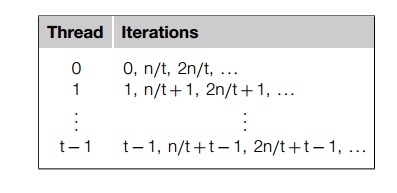
threads. In a cyclic partitioning, the iterations are assigned, one at a time,
in a “round-robin” fashion to the threads. Suppose t = thread_count. Then a cyclic partitioning will assign the iterations as follows:
To get a feel for how drastically this can
affect performance, we wrote a program in which we defined
double f(int i) {
int j, start = i *(i+1)/2, finish = start + i;
double return_val = 0.0;
for (j = start; j <= finish; j++) {
return_val += sin(j);
}
return return_val;
} /* f */
The call f (i) calls the sine function i times, and, for example, the time to execute f (2i) requires approximately twice as much time as
the time to execute f (i).
When we ran the program with n = 10,000 and one thread, the run-time was 3.67
seconds. When we ran the program with two threads and the default assignment—
iterations 0–5000 on thread 0 and iterations 5001–10,000 on thread 1—the
run-time was 2.76 seconds. This is a speedup of only 1.33. However, when we ran
the program with two threads and a cyclic assignment, the run-time was
decreased to 1.84 seconds. This is a speedup of 1.99 over the one-thread run
and a speedup of 1.5 over the two-thread block partition!
We can see that a good assignment of iterations
to threads can have a very sig-nificant effect on performance. In OpenMP,
assigning iterations to threads is called scheduling, and the schedule clause can be used to assign iterations in either a parallel for
or a for directive.
1. The schedule clause
In our example, we already know how to obtain
the default schedule: we just add a parallel
for directive with a reduction clause:
sum = 0.0;
# pragma omp parallel for num_threads(thread_count) \
reduction(+:sum)
for (i =
0; i <= n; i++) sum += f(i);
To get a cyclic schedule, we can add a schedule clause to the parallel for directive:
sum = 0.0;
# pragma omp parallel for num threads(thread count) \
reduction(+:sum) schedule(static,1)
for (i =
0; i <= n; i++) sum += f(i);
In general, the schedule clause has the form
schedule(<type> [, <chunksize>])
The type can be any one of the following:
.. static. The iterations can be assigned to the threads
before the loop is executed. dynamic or guided.
The iterations are assigned to the threads
while the loop is executing, so after a thread completes its
current set of iterations, it can request . more from the run-time
system.
. auto. The compiler and/or the run-time system
determine the schedule. runtime. The schedule is determined at run-time.
The chunksize is a positive integer. In OpenMP parlance, a chunk of iterations is a block of iterations that
would be executed consecutively in the serial loop. The number of iterations in
the block is the chunksize. Only static, dynamic, and guided schedules can have a chunksize. This determines the details of the schedule, but its exact interpretation depends on the type.
2. The static schedule type
For a static schedule, the system assigns chunks of chunksize iterations to each thread in a round-robin fashion. As an example,
suppose we have 12 iterations, 0, 1, ...., 11, and three threads. Then if schedule(static,1) is used in the parallel for or for directive, we’ve already seen that the iterations will be assigned
as
Thread 0 : 0,
3, 6, 9
Thread 1 : 1,
4, 7, 10
Thread 2 : 2,
5, 8, 11
If schedule(static,2) is used, then the iterations will be assigned
as
Thread 0 : 0,
1, 6, 7
Thread 1 : 2,
3, 8, 9
Thread 2 : 4,
5, 10, 11
If schedule(static,4) is used, the iterations will be assigned as
Thread 0 : 0,
1, 2, 3
Thread 1 : 4,
5, 6, 7
Thread 2 : 8,
9, 10, 11
Thus the clause schedule(static, total iterations/thread_count) is more or less equivalent to the default
schedule used by most implementations of OpenMP.
The chunksize can be omitted. If it is omitted, the chunksize is approximately total_iterations/thread
count.
3. The dynamic and guided schedule types
In a dynamic schedule, the iterations are also broken up
into chunks of chunksize consecutive iterations. Each thread executes a
chunk, and when a thread finishes a chunk, it requests another one from the
run-time system. This continues until all the iterations are completed. The chunksize can be omitted. When it is omitted, a chunksize of 1 is used.
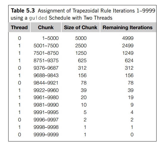
In a guided schedule, each thread also executes a chunk,
and when a thread fin-ishes a chunk, it requests another one. However, in a guided schedule, as chunks are completed, the size of the new chunks
decreases. For example, on one of our systems, if we run the trapezoidal rule
program with the parallel for directive and a schedule(guided) clause, then when n = 10,000 and thread_count = 2, the iterations are assigned as shown in
Table 5.3. We see that the size of the chunk is approximately the number of
iterations remaining divided by the number of threads. The first chunk has size
9999=2~~ 5000, since there are 9999 unassigned iterations. The second
chunk has size 4999=2 ~~2500, and so on.
In a guided schedule, if no chunksize is specified, the size of the chunks decreases
down to 1. If chunksize is specified, it decreases down to chunksize, with the exception that the very last chunk
can be smaller than chunksize.
4. The runtime schedule type
To understand schedule(runtime) we need to digress for a moment and talk about
environment
variables. As the name suggests,
environment variables are named values that can be accessed by a running program. That is, they’re
available in the program’s environment. Some commonly used environment variables are PATH, HOME, and SHELL. The PATH variable specifies which directories the shell
should search when it’s looking for an executable. It’s usually defined in both
Unix and Win-dows. The HOME variable specifies the location of the user’s
home directory, and the SHELL variable specifies the location of the
executable for the user’s shell. These are usually defined in Unix systems. In both
Unix-like systems (e.g., Linux and Mac OS X) and Windows, environment variables
can be examined and specified on the command line. In Unix-like systems, you
can use the shell’s command line.
In Windows systems, you can use the command
line in an integrated development environment.
As an example, if we’re using the bash shell,
we can examine the value of an environment variable by typing
$ echo $PATH
and we can use the export command to set the value of an environment variable
$ export TEST_VAR="hello"
For details about how to examine and set environment
variables for your particular system, you should consult with your local
expert.
When schedule(runtime) is specified, the system uses the environment
vari-able OMP_SCHEDULE to determine at run-time how to schedule the loop. The OMP_SCHEDULE environment variable can take on any of the values that can be used for a static, dynamic, or guided schedule. For example, suppose we
have a parallel for directive in a program and it has been modified by schedule(runtime). Then if we use the bash shell, we can get a cyclic assignment of
iterations to threads by executing the command
$ export OMP_SCHEDULE="static,1"
Now, when we start executing our program, the
system will schedule the iterations of the for loop as if we had the clause schedule(static,1) modifiying the parallel for directive.
5. Which schedule?
If we have a for loop that we’re able to parallelize, how do we decide which type
of schedule we should use and what the chunksize should be? As you may have guessed, there is some overhead associated with the use of a schedule clause. Fur-thermore, the overhead is greater for dynamic schedules than static schedules, and the overhead associated with guided schedules is the greatest of the three. Thus, if we’re getting
satisfactory performance without a schedule clause, we should go no further. However, if
we suspect that the performance of the default schedule can be substantially
improved, we should probably experiment with some different schedules.
In the example at the beginning of this section,
when we switched from the default schedule to schedule(static,1), the speedup of the two-threaded execu-tion of the program
increased from 1.33 to 1.99. Since it’s extremely unlikely that we’ll get speedups that are significantly better
than 1.99, we can just stop here, at least if we’re only going to use two
threads with 10,000 iterations. If we’re going to be using varying numbers of
threads and varying numbers of iterations, we need to do more experimentation,
and it’s entirely possible that we’ll find that the optimal schedule depends on
both the number of threads and the number of iterations.
It can also happen that we’ll decide that the
performance of the default schedule isn’t very good, and we’ll proceed to
search through a large array of schedules and iteration counts only to conclude
that our loop doesn’t parallelize very well and no schedule is going to give us much improved performance. For an
example of this, see Programming Assignment 5.4.
There are some situations in which it’s a good
idea to explore some schedules
.before others:
If each iteration of the loop requires roughly
the same amount of computation, then it’s likely that the default
distribution will give the best performance.
If the cost of the iterations decreases (or
increases) linearly as the loop exe-cutes, then a static schedule with small chunksizes will probably give the best performance.
If the cost of each iteration can’t be
determined in advance, then it may make sense to explore a variety of
scheduling options. The schedule(runtime) clause can be used here, and the different
options can be explored by running the program with different assignments to
the environment variable OMP_SCHEDULE.
Related Topics