Quantity Theories of Money

Quantity Theories of Money

Quantity theories of money explain the relationship between quantity of money and value of money. Here, we are given two approaches of Quantity Theory of Money, viz. Fisher’s Transaction Approach and Cambridge Cash Balance Approach.

(a) Fisher’s Quantity Theory of Money:

The quantity theory of money is a very old theory. It was first propounded in 1588 by an Italian economist, Davanzatti. But, the credit for popularizing this theory in recent years rightly belongs to the well-known American economist, Irving Fisher who published his book, ‘The Purchasing Power of Money” in 1911.He gave it a quantitative form in terms of his famous “Equation of Exchange”.

The general form of equation given by Fisher is

MV = PT

Where M = Money Supply/quantity of Money

V = Velocity of Money

P = Price level

T = Volume of Transaction.

Fisher points out that in a country during any given period of time, the total quantity of money (MV) will be equal to the total value of all goods and services bought and sold (PT).

MV = PT

Supply of Money = Demand for Money

This equation is referred to as “Cash Transaction Equation”.

It is expressed as P = MV / T which implies that the quantity of money determines the price level and the price level in its turn varies directly with the quantity of money, provided ‘V’ and ‘T’ remain constant.

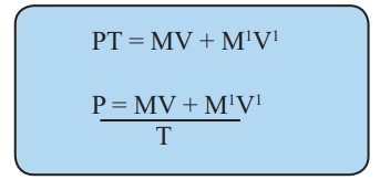
The above equation considers only currency money. But, in a modern economy, bank’s demand deposits or credit money and its velocity play a vital part in business. Therefore, Fisher extended his original equation of exchange to include bank deposits M1 and its velocity V1. The revised equation was:

PT = MV + M¹V1

P = [ MV + M¹V¹] / T

From the revised equation, it is evident, that the price level is determined by

(a) the quantity of money in circulation ‘M’

(b) the velocity of circulation of money ‘V’

(c) the volume of bank credit money M₁

(d) the velocity of circulation of credit money V₁ and the volume of trade (T)

Diagrammatic Illustration

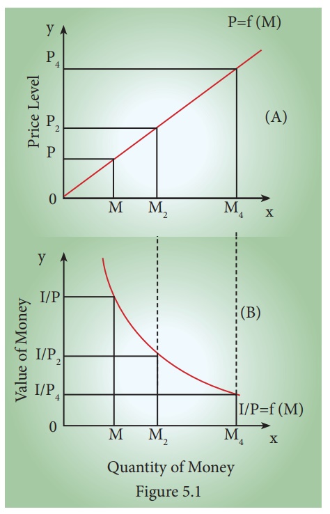
Figure (A) shows the effect of changes in the quantity of money on the price level. When the quantity of money is OM, the price level is OP. When the quantity of money is doubled to OM₂ , the price level is also doubled to OP ₂ . Further, when the quantity of money is increased four-fold to OM₄ , the price level also increases by four times to OP₄ . This relationship is expressed by the curve OP = f (M) from the origin at 450.

Figure (B), shows the inverse relation between the quantity of money and the value of money, where the value of money is taken on the vertical axis. When the quantity of money is OM, the value of money is OI / P. But with the doubling of the quantity of money to OM₂ , the value of money becomes one-half of what it was before, (OI / P₂). But, with the quantity of money increasing by four-fold to OM₄, the value of money is reduced by OI / P₄. This inverse relationship between the quantity of money and the value of money is shown by downward sloping curve IO / P = f(M).

b) Cambridge Approach (Cash Balances Approach)

i) Marshall’s Equation

The Marshall equation is expressed as:

M = KPY

Where

M is the quantity of money

Y is the aggregate real income of the community

P is Purchasing Power of money

K represents the fraction of the real income which the public desires to hold in the form of money.

Thus, the price level P = M/KY or the value of money (The reciprocal of price level) is 1/P = KY/M

The value of money in terms of this equation can be found out by dividing the total quantity of goods which the public desires to holdout of the total income by the total supply of money.

According to Marshall’s equation, the value of money is influenced not only by changes in M, but also by changes in K.

ii) Keynes’ Equation

Keynes equation is expressed as:

n = pk (or) p = n / k

Where

n is the total supply of money

p is the general price level of consumption goods

k is the total quantity of consumption units the people decide to keep in the form of cash,

Keynes indicates that K is a real balance, because it is measured in terms of consumer goods.

According to Keynes, peoples’ desire to hold money is unaltered by monetary authority. So, price level and value of money can be stabilized through regulating quantity of money (n) by the monetary authority.

Later, Keynes extended his equation in the following form:

n = p (k + rk') or p = n/(k + rk')

Where,

n = total money supply

p = price level of consumer goods

k = peoples' desire to hold money in hand (in terms of consumer goods) in the total income of them

r = cash reserve ratio

k' = community’s total money deposit in banks, in terms of consumers goods.

In this extended equation also, Keynes assumes that, k, k' and r are constant. In this situation, price level (P) is changed directly and proportionately changing in money volume (n).