Polynomial Solutions and Straight Beams

Polynomial Solutions and Straight Beams

A number of stress fields in rectangular coordinates will be presented or asked for in problems in later pages. In most cases, these results are obtained most easily by solving in polar coordinates and transforming them to Cartesian form by Mohr’s Circle. However for beams (long rectan-gular strips) polynomial stress functions in Cartesian coordinates are pref-erable because boundary conditions are easily expressed. It is also possible to compare the more exact elasticity solutions thus generated directly to the standard strength-of-materials type solutions,* which are expressed in powers of x and y. To get ahead of ourselves, we will show that, away from concen-trated loads or support reactions (which are a separate problem), the elasticity modifications of elementary formulae are significant for design only for very short beams (where the span and depth are comparable).

A polynomial of n^th degree with unknown coefficients can be written:

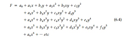
The constant a₀ and first-order terms give no stresses and can be omitted. The second-order terms give constant stress components and the third-order terms, linear stress components corresponding to the free fields of Chapter 5. Since the polynomial terms through the third order automatically satisfy the biharmonic equation Ɐ⁴F  =  0, the unknown coefficients can be adjusted at will to satisfy the boundary conditions.* However, for polynomials of higher than third degree, there must be relationships between the coefficients if geo-metric compatibility, expressed by Equation (6.3), is to be maintained. For example, if all the fourth-order terms were included, then Equation (6.3) would be satisfied only if:

a₄ + 2c₄  +  e₄ = 0

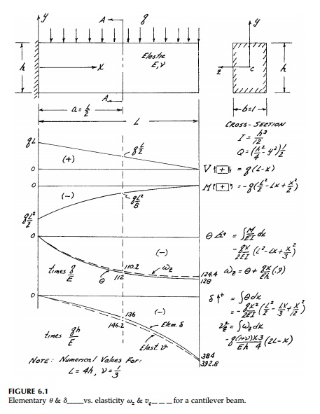
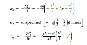
Consider, for example, the case of a cantilever beam with a uniform load as shown in Figure 6.1. Using the strength-of-materials approach based on plane sections, gives the elementary formulas:

Let us now develop an elasticity solution using a polynomial stress func-tion and the semi-inverse approach of rational mechanics in choosing appro-priate terms. There are two stress boundary conditions on each of the three exposed faces and two overall equilibrium conditions at x = 0. We will also get an equation relating coefficients from Equation (6.3). Thus we should apparently assume a polynomial with at least nine terms. From our physical understanding, we know we should not include terms with even powers of y greater than two since σ_y changes sign top and bottom. Also, since σ_y should not vary with x, we should eliminate all xⁿ > x². Therefore, starting with the second-order terms, assume the stress function.

F = a₂ x² + b₂ xy + b₃ x² y + c₃ xy² + d₃ y³  + c₄ x² y² + d₄ xy³ + d₅ x² y³ +  f ₅ y⁵     (6.5)

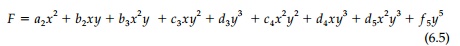
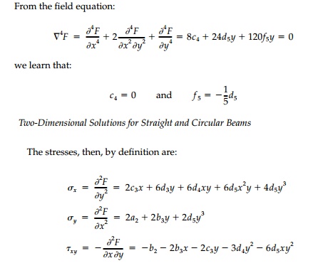
Looking at σ_x and τ_xy, it is clear that the c₃ term is unrealistic. There should not be a large normal stress at the neutral axis (y = 0) or a linear shear term that changes sign. Therefore let c₃ = 0

Applying the boundary conditions at the top and bottom:

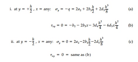
While it looks like we are losing a boundary condition, the x = any require-ment on

 (b) gives two requirements:

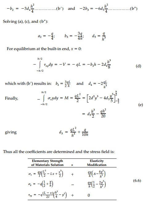
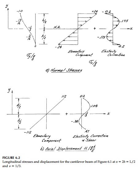
The shear stress distribution is exactly that given by the elementary for-mula. The “elasticity correction” to σ_x is plotted in Figure 6.2a, as is the dis-tribution of σ_y , which is not considered at all in the elementary theory. Both are independent of x so that at x = L the boundary condition, that the end of the beam be free of normal stresses, is not satisfied.* However, these stresses are very small and the net resultant ʃσ_x dA is in fact zero so that only very close to the end of the beam will this elasticity correction be inexact.

Note that σ_y and the elasticity correction to σ_x are plotted in Figure 6.2a at greatly exaggerated scale so they are recognizable compared to the basic ele-mentary portion of σ_x. In practice they are of no engineering significance. At x=0, where σ_x will be maximum when y =+ -  h/2

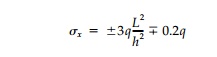
Even for a very short beam, say L = 2h, the elasticity contribution is less than 2%. Other uncertainties introduced by the geometric conditions of a real built-in support at x = 0 (not rigid and not plane stress) would be more important.

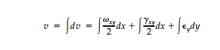
The deflection of the beam can be determined by integrating the relative displacements given by Equation (4.18). From the stress�'strain relation-ships:

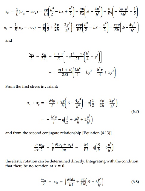
The first term, being the integral of the moment diagram, is the same as the slope, θ, given by elementary theory and the second, the elasticity contribu-tion, is due primarily to σ_y now being included. Substituting the expression for the Moment Diagram:

Since this is plane stress, there will be elastic rotation ω_x and anticlastic cur-vature, but we will concern ourselves with the displacement of the centroidal plane of symmetry z = 0.

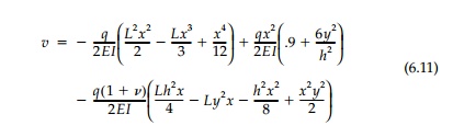
The displacements are found by integrating Equation (4.17) directly with the support condition that at x = 0 and y = any, u = v = 0.

The first term not in the elementary theory is the Poisson-ratio effect due to (σ_y)_avg = - q/2 giving (E_x)_avg = + υq/2E which integrates to a linear function of x. The second term, linear in y, conforms with the assumption of plane sec-tions with the last two h² components being a contribution from elasticity. The final y³ term warps the cross-section and is a result of E_y, the elasticity correc-tion to E_x and the shear strain γ_xy , all of which are not included in the elemen-tary solution for displacements. The warping of an arbitrary cross-section at x = a = 2h for a short beam L = 4h is shown in Figure 6.2b. It is clear that from an engineering standpoint the elementary formula is perfectly adequate.

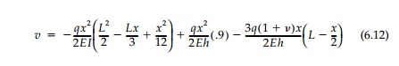
Following the same procedure to find the vertical displacement

where the third term does not contribute directly since v must equal zero at x = 0. Therefore:

The first term is the integral of the slope diagram as in the elementary the-ory, and the second and third terms are the contributions from the elasticity correction and the shear, respectively. The deflection of the centroidal axis at y = 0 is therefore:

The rotation ω_z and vertical deflection v of the centroidal axis from elasticity are compared to the values for θ and ς from elementary theory in Figure 6.1. As was true for stresses and longitudinal displacements, the difference between them must be exaggerated in plotting to be recognizable.

This conclusion that elementary analysis for straight beams is very accurate will be true for all other cases of distributed loading. Therefore, while most texts include a few more examples, here they are left to the chapter prob-lems. Some further remarks concerning straight beams are included in the final section.

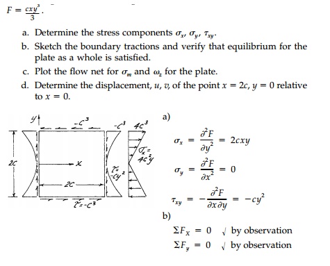
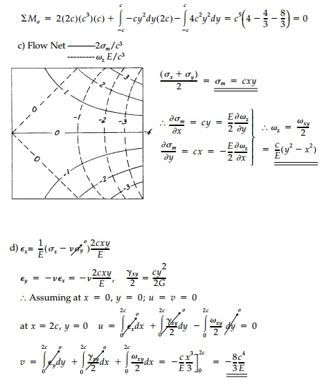
Example 6.1

A thin elastic square plate of 2c on a side is free of body forces and is subjected to a loading around its four edges such that the stress function is found to be