Other Types of Indexes

Other Types of Indexes

1. Hash Indexes

It is also possible to create access structures similar to indexes that are based on hashing. The hash index is a secondary structure to access the file by using hashing on a search key other than the one used for the primary data file organization. The index entries are of the type <K, Pr> or <K, P>, where Pr is a pointer to the record containing the key, or P is a pointer to the block containing the record for that key. The index file with these index entries can be organized as a dynamically expand-able hash file, using one of the techniques described in Section 17.8.3; searching for an entry uses the hash search algorithm on K. 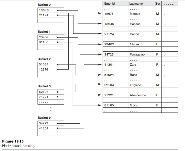Once an entry is found, the pointer Pr (or P) is used to locate the corresponding record in the data file. Figure 18.15 illustrates a hash index on the Emp_id field for a file that has been stored as a sequential file ordered by Name. The Emp_id is hashed to a bucket number by using a hashing function: the sum of the digits of Emp_id modulo 10. For example, to find Emp_id 51024, the hash function results in bucket number 2; that bucket is accessed first. It contains the index entry < 51024, Pr >; the pointer Pr leads us to the actual record in the file. In a practical application, there may be thousands of buckets; the bucket number, which may be several bits long, would be subjected to the directory schemes discussed about dynamic hashing in Section 17.8.3. Other search struc-tures can also be used as indexes.

2. Bitmap Indexes

The bitmap index is another popular data structure that facilitates querying on multiple keys. Bitmap indexing is used for relations that contain a large number of rows. It creates an index for one or more columns, and each value or value range in those columns is indexed. Typically, a bitmap index is created for those columns that contain a fairly small number of unique values. To build a bitmap index on a set of records in a relation, the records must be numbered from 0 to n with an id (a record id or a row id) that can be mapped to a physical address made of a block number and a record offset within the block.

A bitmap index is built on one particular value of a particular field (the column in a relation) and is just an array of bits. Consider a bitmap index for the column C and a value V for that column. For a relation with n rows, it contains n bits. The i^th bit is set to 1 if the row i has the value V for column C; otherwise it is set to a 0. 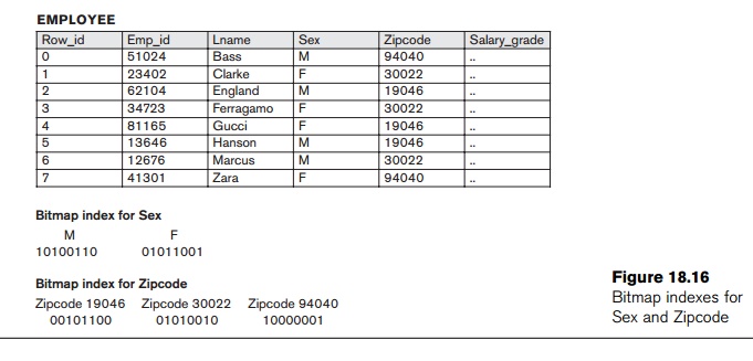If C contains the valueset <v₁, v₂, ..., v_m> with m distinct values, then m bitmap indexes would be created for that column. Figure 18.16 shows the relation EMPLOYEE with columns Emp_id, Lname, Sex, Zipcode, and Salary_grade (with just 8 rows for illustra-tion) and a bitmap index for the Sex and Zipcode columns. As an example, if the bitmap for Sex = F, the bits for Row_ids 1, 3, 4, and 7 are set to 1, and the rest of the bits are set to 0, the bitmap indexes could have the following query applications:

For the query C₁ = V₁ , the corresponding bitmap for value V₁ returns the Row_ids containing the rows that qualify.

        For the query C₁= V₁ and C₂ = V₂ (a multikey search request), the two cor-responding bitmaps are retrieved and intersected (logically AND-ed) to yield the set of Row_ids that qualify. In general, k bitvectors can be intersected to deal with k equality conditions. Complex AND-OR conditions can also be supported using bitmap indexing.

        To retrieve a count of rows that qualify for the condition C₁ = V₁, the “1” entries in the corresponding bitvector are counted.

        Queries with negation, such as C₁ ¬ = V₁, can be handled by applying the Boolean complement operation on the corresponding bitmap.

Consider the example in Figure 18.16. To find employees with Sex = F and Zipcode = 30022, we intersect the bitmaps “01011001” and “01010010” yielding Row_ids 1 and 3. Employees who do not live in Zipcode = 94040 are obtained by complementing the bitvector “10000001” and yields Row_ids 1 through 6. In general, if we assume uniform distribution of values for a given column, and if one col-umn has 5 distinct values and another has 10 distinct values, the join condition on these two can be considered to have a selectivity of 1/50 (=1/5 _* 1/10). Hence, only about 2 percent of the records would actually have to be retrieved. If a column has only a few values, like the Sex column in Figure 18.16, retrieval of the Sex = M condition on average would retrieve 50 percent of the rows; in such cases, it is better to do a complete scan rather than use bitmap indexing.

In general, bitmap indexes are efficient in terms of the storage space that they need. If we consider a file of 1 million rows (records) with record size of 100 bytes per row, each bitmap index would take up only one bit per row and hence would use 1 mil-lion bits or 125 Kbytes. Suppose this relation is for 1 million residents of a state, and they are spread over 200 ZIP Codes; the 200 bitmaps over Zipcodes contribute 200 bits (or 25 bytes) worth of space per row; hence, the 200 bitmaps occupy only 25 percent as much space as the data file. They allow an exact retrieval of all residents who live in a given ZIP Code by yielding their Row_ids.

When records are deleted, renumbering rows and shifting bits in bitmaps becomes expensive. Another bitmap, called the existence bitmap, can be used to avoid this expense. This bitmap has a 0 bit for the rows that have been deleted but are still present and a 1 bit for rows that actually exist. Whenever a row is inserted in the relation, an entry must be made in all the bitmaps of all the columns that have a bitmap index; rows typically are appended to the relation or may replace deleted rows. This process represents an indexing overhead.

Large bitvectors are handled by treating them as a series of 32-bit or 64-bit vectors, and corresponding AND, OR, and NOT operators are used from the instruction set to deal with 32- or 64-bit input vectors in a single instruction. This makes bitvector operations computationally very efficient.

Bitmaps for B⁺-Tree Leaf Nodes. Bitmaps can be used on the leaf nodes of B⁺-tree indexes as well as to point to the set of records that contain each specific value of the indexed field in the leaf node. When the B⁺-tree is built on a nonkey search field, the leaf record must contain a list of record pointers alongside each value of the indexed attribute. For values that occur very frequently, that is, in a large percentage of the relation, a bitmap index may be stored instead of the pointers. As an example, for a relation with n rows, suppose a value occurs in 10 percent of the file records. A bitvector would have n bits, having the “1” bit for those Row_ids that contain that search value, which is n/8 or 0.125n bytes in size. If the record pointer takes up 4 bytes (32 bits), then the n/10 record pointers would take up 4 _* n/10 or 0.4n bytes. Since 0.4n is more than 3 times larger than 0.125n, it is better to store the bitmap index rather than the record pointers. Hence for search values that occur more frequently than a certain ratio (in this case that would be 1/32), it is beneficial to use bitmaps as a compressed storage mechanism for representing the record pointers in B⁺-trees that index a nonkey field.

3. Function-Based Indexing

In this section we discuss a new type of indexing, called function-based indexing, that has been introduced in the Oracle relational DBMS as well as in some other commercial products.

The idea behind function-based indexing is to create an index such that the value that results from applying some function on a field or a collection of fields becomes the key to the index. The following examples show how to create and use function-based indexes.

Example 1. The following statement creates a function-based index on the EMPLOYEE table based on an uppercase representation of the Lname column, which can be entered in many ways but is always queried by its uppercase representation.

CREATE INDEX upper_ix ON Employee (UPPER(Lname));

This statement will create an index based on the function UPPER(Lname), which returns the last name in uppercase letters; for example, UPPER('Smith') will return ‘SMITH’.

Function-based indexes ensure that Oracle Database system will use the index rather than perform a full table scan, even when a function is used in the search predicate of a query. For example, the following query will use the index:

SELECT First_name, Lname

FROM Employee

WHERE UPPER(Lname)= "SMITH".

Without the function-based index, an Oracle Database might perform a full table scan, since a B⁺-tree index is searched only by using the column value directly; the use of any function on a column prevents such an index from being used.

Example 2. In this example, the EMPLOYEE table is supposed to contain two fields—salary and commission_pct (commission percentage)—and an index is being created on the sum of salary and commission based on the commission_pct.

CREATE INDEX income_ix

ON Employee(Salary + (Salary*Commission_pct));

The following query uses the income_ix index even though the fields salary and commission_pct are occurring in the reverse order in the query when compared to the index definition.

SELECT First_name, Lname

FROM Employee

WHERE ((Salary*Commission_pct) + Salary ) > 15000;

Example 3. This is a more advanced example of using function-based indexing to define conditional uniqueness. The following statement creates a unique function-based index on the ORDERS table that prevents a customer from taking advantage of a promotion id (“blowout sale”) more than once. It creates a composite index on the Customer_id and Promotion_id fields together, and it allows only one entry in the index for a given Customer_id with the Promotion_id of “2” by declaring it as a unique index.

CREATE UNIQUE INDEX promo_ix ON Orders

(CASE WHEN Promotion_id = 2 THEN Customer_id ELSE NULL END, CASE WHEN Promotion_id = 2 THEN Promotion_id ELSE NULL END);

Note that by using the CASE statement, the objective is to remove from the index any rows where Promotion_id is not equal to 2. Oracle Database does not store in the B⁺-tree index any rows where all the keys are NULL. Therefore, in this example, we map both Customer_id and Promotion_id to NULL unless Promotion_id is equal to 2. The result is that the index constraint is violated only if Promotion_id is equal to 2, for two (attempted insertions of) rows with the same Customer_id value.