Dynamic Multilevel Indexes Using B-Trees and B+-Trees

Dynamic Multilevel Indexes Using B-Trees and B⁺-Trees

B-trees and B⁺-trees are special cases of the well-known search data structure known as a tree. We briefly introduce the terminology used in discussing tree data structures. A tree is formed of nodes. Each node in the tree, except for a special node called the root, has one parent node and zero or more child nodes. The root node has no parent. A node that does not have any child nodes is called a leaf node; a nonleaf node is called an internal node. The level of a node is always one more than the level of its parent, with the level of the root node being zero.⁵ A subtree of a node consists of that node and all its descendant nodes—its child nodes, the child nodes of its child nodes, and so on. A precise recursive definition of a subtree is that it consists of a node n and the subtrees of all the child nodes of n. 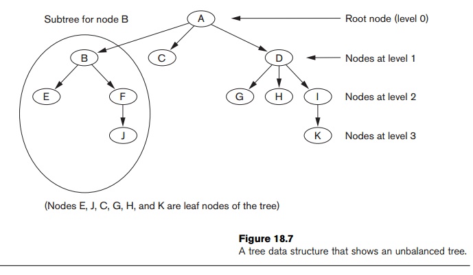Figure 18.7 illustrates a tree data structure. In this figure the root node is A, and its child nodes are B, C, and D. Nodes E, J, C, G, H, and K are leaf nodes. Since the leaf nodes are at different levels of the tree, this tree is called unbalanced.

In Section 18.3.1, we introduce search trees and then discuss B-trees, which can be used as dynamic multilevel indexes to guide the search for records in a data file. B-tree nodes are kept between 50 and 100 percent full, and pointers to the data blocks are stored in both internal nodes and leaf nodes of the B-tree structure. In Section 18.3.2 we discuss B⁺-trees, a variation of B-trees in which pointers to the data blocks of a file are stored only in leaf nodes, which can lead to fewer levels and higher-capacity indexes. In the DBMSs prevalent in the market today, the common structure used for indexing is B⁺-trees.

1. Search Trees and B-Trees

A search tree is a special type of tree that is used to guide the search for a record, given the value of one of the record’s fields. The multilevel indexes discussed in Section 18.2 can be thought of as a variation of a search tree; each node in the multilevel index can have as many as fo pointers and fo key values, where fo is the index fan-out. The index field values in each node guide us to the next node, until we reach the data file block that contains the required records. By following a pointer, we restrict our search at each level to a subtree of the search tree and ignore all nodes not in this subtree.

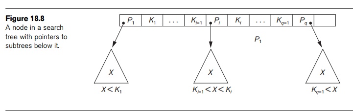
Search Trees. A search tree is slightly different from a multilevel index. A search tree of order p is a tree such that each node contains at most p − 1 search values and p pointers in the order <P₁, K₁, P₂, K₂, ..., P_q−1, K_q−1, P_q>, where q ≤ p. Each P_i is a pointer to a child node (or a NULL pointer), and each K_i is a search value from some ordered set of values. All search values are assumed to be unique.⁶ Figure 18.8 illustrates a node in a search tree. Two constraints must hold at all times on the search tree:

        Within each node, K₁ < K₂ < ... < K_q−1.

        For all values X in the subtree pointed at by P_i, we have K_i−1 < X < K_i for 1 <

i < q; X < K_i for i = 1; and K_i−1 < X for i = q (see Figure 18.8).

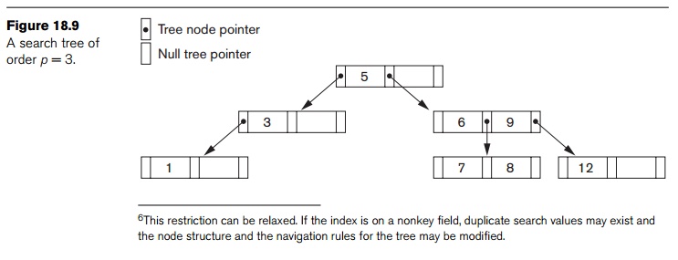
Whenever we search for a value X, we follow the appropriate pointer P_i according to the formulas in condition 2 above. Figure 18.9 illustrates a search tree of order p = 3 and integer search values. Notice that some of the pointers P_i in a node may be NULL pointers.

We can use a search tree as a mechanism to search for records stored in a disk file. The values in the tree can be the values of one of the fields of the file, called the search field (which is the same as the index field if a multilevel index guides the search). Each key value in the tree is associated with a pointer to the record in the data file having that value. Alternatively, the pointer could be to the disk block containing that record. The search tree itself can be stored on disk by assigning each tree node to a disk block. When a new record is inserted in the file, we must update the search tree by inserting an entry in the tree containing the search field value of the new record and a pointer to the new record.

Algorithms are necessary for inserting and deleting search values into and from the search tree while maintaining the preceding two constraints. In general, these algorithms do not guarantee that a search tree is balanced, meaning that all of its leaf nodes are at the same level. The tree in Figure 18.7 is not balanced because it has leaf nodes at levels 1, 2, and 3. The goals for balancing a search tree are as follows:

                                 To guarantee that nodes are evenly distributed, so that the depth of the tree is minimized for the given set of keys and that the tree does not get skewed with some nodes being at very deep levels

                                         To make the search speed uniform, so that the average time to find any random key is roughly the same

While minimizing the number of levels in the tree is one goal, another implicit goal is to make sure that the index tree does not need too much restructuring as records are inserted into and deleted from the main file. Thus we want the nodes to be as full as possible and do not want any nodes to be empty if there are too many deletions. Record deletion may leave some nodes in the tree nearly empty, thus wasting storage space and increasing the number of levels. The B-tree addresses both of these problems by specifying additional constraints on the search tree.

B-Trees. The B-tree has additional constraints that ensure that the tree is always balanced and that the space wasted by deletion, if any, never becomes excessive. The algorithms for insertion and deletion, though, become more complex in order to maintain these constraints. Nonetheless, most insertions and deletions are simple processes; they become complicated only under special circumstances—namely, whenever we attempt an insertion into a node that is already full or a deletion from a node that makes it less than half full. More formally, a B-tree of order p, when used as an access structure on a key field to search for records in a data file, can be defined as follows:

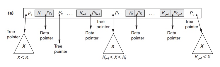
1. Each internal node in the B-tree (Figure 18.10(a)) is of the form

<P₁, <K₁, Pr₁>, P₂, <K₂, Pr₂>, ..., <K_q–1, Pr_q–1>, P_q>

where q ≤ p. Each P_i is a tree pointer—a pointer to another node in the B-tree. Each Pr_i is a data pointer⁸—a pointer to the record whose search key field value is equal to K_i (or to the data file block containing that record).

   2. Within each node, K₁ < K₂ < ... < K_q−1.

        3. For all search key field values X in the subtree pointed at by P_i (the ith sub-tree, see Figure 18.10(a)), we have:

K_i–1 < X < K_i for 1 < i < q; X < K_i for i = 1; and K_i–1 < X for i = q. 

  4. Each node has at most p tree pointers.

        5. Each node, except the root and leaf nodes, has at least (p/2) tree pointers. The root node has at least two tree pointers unless it is the only node in the tree.

        6. A node with q tree pointers, q ≤ p, has q – 1 search key field values (and hence has q – 1 data pointers).

        7. All leaf nodes are at the same level. Leaf nodes have the same structure as internal nodes except that all of their tree pointers P_i are NULL.

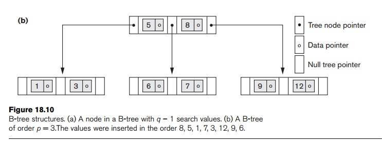
Figure 18.10(b) illustrates a B-tree of order p = 3. Notice that all search values K in the B-tree are unique because we assumed that the tree is used as an access structure on a key field. If we use a B-tree on a nonkey field, we must change the definition of the file pointers Pr_i to point to a block—or a cluster of blocks—that contain the pointers to the file records. This extra level of indirection is similar to option 3, dis-cussed in Section 18.1.3, for secondary indexes.

 A B-tree starts with a single root node (which is also a leaf node) at level 0 (zero). Once the root node is full with p – 1 search key values and we attempt to insert another entry in the tree, the root node splits into two nodes at level 1. Only the middle value is kept in the root node, and the rest of the values are split evenly between the other two nodes. When a nonroot node is full and a new entry is inserted into it, that node is split into two nodes at the same level, and the middle entry is moved to the parent node along with two pointers to the new split nodes. If the parent node is full, it is also split. Splitting can propagate all the way to the root node, creating a new level if the root is split. We do not discuss algorithms for B-trees in detail in this book,⁹ but we outline search and insertion procedures for B⁺-trees in the next section.

If deletion of a value causes a node to be less than half full, it is combined with its neighboring nodes, and this can also propagate all the way to the root. Hence, deletion can reduce the number of tree levels. It has been shown by analysis and simulation that, after numerous random insertions and deletions on a B-tree, the nodes are approximately 69 percent full when the number of values in the tree stabilizes. This is also true of B⁺-trees. If this happens, node splitting and combining will occur only rarely, so insertion and deletion become quite efficient. If the number of values grows, the tree will expand without a problem—although splitting of nodes may occur, so some insertions will take more time. Each B-tree node can have at most p tree pointers, p – 1 data pointers, and p – 1 search key field values (see Figure 18.10(a)).

In general, a B-tree node may contain additional information needed by the algorithms that manipulate the tree, such as the number of entries q in the node and a pointer to the parent node. Next, we illustrate how to calculate the number of blocks and levels for a B-tree.

Example 4. Suppose that the search field is a nonordering key field, and we con-struct a B-tree on this field with p = 23. Assume that each node of the B-tree is 69 percent full. Each node, on the average, will have p _* 0.69 = 23 _* 0.69 or approximately 16 pointers and, hence, 15 search key field values. The average fan-out fo = 16. We can start at the root and see how many values and pointers can exist, on the average, at each subsequent level:

Root: 1 node         15 key entries       16 pointers

Level 1:       16 nodes     240 key entries     256 pointers

Level 2:       256 nodes   3840 key entries   4096 pointers

Level 3:       4096 nodes 61,440 key entries        

At each level, we calculated the number of key entries by multiplying the total number of pointers at the previous level by 15, the average number of entries in each node. Hence, for the given block size, pointer size, and search key field size, a two-level B-tree holds 3840 + 240 + 15 = 4095 entries on the average; a three-level B-tree holds 65,535 entries on the average.

B-trees are sometimes used as primary file organizations. In this case, whole records are stored within the B-tree nodes rather than just the <search key, record pointer> entries. This works well for files with a relatively small number of records and a small record size. Otherwise, the fan-out and the number of levels become too great to permit efficient access.

In summary, B-trees provide a multilevel access structure that is a balanced tree structure in which each node is at least half full. Each node in a B-tree of order p can have at most p − 1 search values.

2. B⁺-Trees

Most implementations of a dynamic multilevel index use a variation of the B-tree data structure called a B⁺-tree. In a B-tree, every value of the search field appears once at some level in the tree, along with a data pointer. In a B⁺-tree, data pointers are stored only at the leaf nodes of the tree; hence, the structure of leaf nodes differs from the structure of internal nodes. The leaf nodes have an entry for every value of the search field, along with a data pointer to the record (or to the block that contains this record) if the search field is a key field. For a nonkey search field, the pointer points to a block containing pointers to the data file records, creating an extra level of indirection.

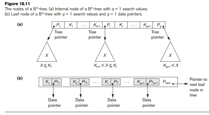
The leaf nodes of the B⁺-tree are usually linked to provide ordered access on the search field to the records. These leaf nodes are similar to the first (base) level of an index. Internal nodes of the B⁺-tree correspond to the other levels of a multilevel index. Some search field values from the leaf nodes are repeated in the internal nodes of the B⁺-tree to guide the search. The structure of the internal nodes of a B⁺-tree of order p (Figure 18.11(a)) is as follows:

1. Each internal node is of the form

<P₁, K₁, P₂, K₂, ..., P_{q – 1}, K_{q –1}, P_q> where q ≤ p and each P_i is a tree pointer.

        Within each internal node, K₁ < K₂ < ... < K_q−1.

        For all search field values X in the subtree pointed at by P_i, we have K_i−1 < X ≤ K_i for 1 < i < q; X ≤ K_i for i = 1; and K_i−1 < X for i = q (see Figure 18.11(a)).¹⁰

        Each internal node has at most p tree pointers.

        Each internal node, except the root, has at least (p/2) tree pointers. The root node has at least two tree pointers if it is an internal node.

        An internal node with q pointers, q ≤ p, has q − 1 search field values.

The structure of the leaf nodes of a B⁺-tree of order p (Figure 18.11(b)) is as follows:

1. Each leaf node is of the form

<<K₁, Pr₁>, <K₂, Pr₂>, ..., <K_q–1, Pr_q–1>, P_next>

where q ≤ p, each Pr_i is a data pointer, and P_next points to the next leaf node of the B⁺-tree.

        2. Within each leaf node, K₁ ≤ K₂ ... , K_q−1, q ≤ p.

        3. Each Pr_i is a data pointer that points to the record whose search field value is K_i or to a file block containing the record (or to a block of record pointers that point to records whose search field value is K_i if the search field is not a key).

        4. Each leaf node has at least  (p/2)  values.

        5. All leaf nodes are at the same level.

The pointers in internal nodes are tree pointers to blocks that are tree nodes, whereas the pointers in leaf nodes are data pointers to the data file records or blocks—except for the P_next pointer, which is a tree pointer to the next leaf node. By starting at the leftmost leaf node, it is possible to traverse leaf nodes as a linked list, using the P_next pointers. This provides ordered access to the data records on the indexing field. A P_previous pointer can also be included. For a B⁺-tree on a nonkey field, an extra level of indirection is needed similar to the one shown in Figure 18.5, so the Pr pointers

are block pointers to blocks that contain a set of record pointers to the actual records in the data file, as discussed in option 3 of Section 18.1.3.

Because entries in the internal nodes of a B⁺-tree include search values and tree pointers without any data pointers, more entries can be packed into an internal node of a B⁺-tree than for a similar B-tree. Thus, for the same block (node) size, the order p will be larger for the B⁺-tree than for the B-tree, as we illustrate in Example 5. This can lead to fewer B⁺-tree levels, improving search time. Because the structures for internal and for leaf nodes of a B⁺-tree are different, the order p can be different. We will use p to denote the order for internal nodes and p_leaf to denote the order for leaf nodes, which we define as being the maximum number of data pointers in a leaf node.

Example 5. To calculate the order p of a B⁺-tree, suppose that the search key field is V = 9 bytes long, the block size is B = 512 bytes, a record pointer is Pr = 7 bytes, and a block pointer is P = 6 bytes. An internal node of the B⁺-tree can have up to p tree pointers and p – 1 search field values; these must fit into a single block. Hence, we have:

(p _* P) + ((p – 1) _* V) ≤ B (P _* 6) + ((P − 1) _* 9) ≤ 512 (15 _* p) ≤ 521

We can choose p to be the largest value satisfying the above inequality, which gives p = 34. This is larger than the value of 23 for the B-tree (it is left to the reader to compute the order of the B-tree assuming same size pointers), resulting in a larger fan-out and more entries in each internal node of a B⁺-tree than in the corresponding B-tree. The leaf nodes of the B⁺-tree will have the same number of values and pointers, except that the pointers are data pointers and a next pointer. Hence, the order p_leaf for the leaf nodes can be calculated as follows:

(p_{leaf *} (Pr + V)) + P ≤ B (p_{leaf *} (7 + 9)) + 6 ≤ 512 ⁽¹⁶ * ^p_leaf⁾ ≤ ⁵⁰⁶

It follows that each leaf node can hold up to p_leaf = 31 key value/data pointer combi-nations, assuming that the data pointers are record pointers.

As with the B-tree, we may need additional information—to implement the inser-tion and deletion algorithms—in each node. This information can include the type of node (internal or leaf), the number of current entries q in the node, and pointers to the parent and sibling nodes. Hence, before we do the above calculations for p and p_leaf, we should reduce the block size by the amount of space needed for all such information. The next example illustrates how we can calculate the number of entries in a B⁺-tree.

Example 6. Suppose that we construct a B⁺-tree on the field in Example 5. To calculate the approximate number of entries in the B⁺-tree, we assume that each node is 69 percent full. On the average, each internal node will have 34 _* 0.69 or approximately 23 pointers, and hence 22 values. Each leaf node, on the average, will hold 0.69 _* p_leaf = 0.69 _* 31 or approximately 21 data record pointers. A B⁺-tree will have the following average number of entries at each level:

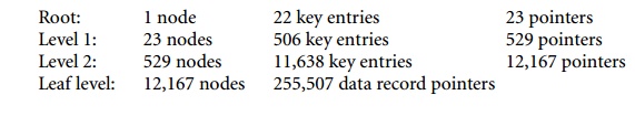
For the block size, pointer size, and search field size given above, a three-level B⁺-tree holds up to 255,507 record pointers, with the average 69 percent occupancy of nodes. Compare this to the 65,535 entries for the corresponding B-tree in Example 4. This is the main reason that B⁺-trees are preferred to B-trees as indexes to data-base files.

Search, Insertion, and Deletion with B⁺-Trees. Algorithm 18.2 outlines the procedure using the B⁺-tree as the access structure to search for a record. Algorithm 18.3 illustrates the procedure for inserting a record in a file with a B⁺-tree access structure. These algorithms assume the existence of a key search field, and they must be modified appropriately for the case of a B⁺-tree on a nonkey field. We illustrate insertion and deletion with an example.

Algorithm 18.2. Searching for a Record with Search Key Field Value K, Using a B⁺-tree

n ← block containing root node of B⁺-tree; read block n;

while (n is not a leaf node of the B⁺-tree) do begin

q ← number of tree pointers in node n;

if K ≤ n.K₁ (*n.K_i refers to the ith search field value in node n*) then n ← n.P₁ (*n.P_i refers to the ith tree pointer in node n*)

else if K > n.K_q−1 then n ← n.P_q else begin

search node n for an entry i such that n.K_i−1 < K ≤n.K_i;

n ← n.P_i end;

read block n end;

search block n for entry (K_i, Pr_i) with K = K_i; (* search leaf node *) if found

then read data file block with address Pr_i and retrieve record else the record with search field value K is not in the data file;

Algorithm 18.3. Inserting a Record with Search Key Field Value K in a B⁺-tree of Order p

n ← block containing root node of B⁺-tree; read block n; set stack S to empty;

while (n is not a leaf node of the B⁺-tree) do begin

push address of n on stack S;

(*stack S holds parent nodes that are needed in case of split*) q ← number of tree pointers in node n;

if K ≤n.K₁ (*n.K_i refers to the ith search field value in node n*)

then n ← n.P₁ (*n.P_i refers to the ith tree pointer in node n*) else if K > n.K_q−1

then n ← n.P_q else begin

search node n for an entry i such that n.K_i−1 < K fn.K_i;

n ← n.P_i end;

read block n

end;

search block n for entry (K_i,Pr_i) with K = K_i; (*search leaf node n*) if found

then record already in file; cannot insert

else (*insert entry in B⁺-tree to point to record*) begin

create entry (K, Pr) where Pr points to the new record; if leaf node n is not full

then insert entry (K, Pr) in correct position in leaf node n

else begin (*leaf node n is full with p_leaf record pointers; is split*) copy n to temp (*temp is an oversize leaf node to hold extra

entries*);

insert entry (K, Pr) in temp in correct position;

(*temp now holds p_leaf + 1 entries of the form (K_i, Pr_i)*)

new ← a new empty leaf node for the tree; new.P_next ← n.P_next ; j ← (p_leaf + 1)/2 ;

n ← first j entries in temp (up to entry (K_j, Pr_j)); n.P_next ← new; new ← remaining entries in temp; K ← K_j ;

(*now we must move (K, new) and insert in parent internal node; however, if parent is full, split may propagate*)

finished ← false; repeat

if stack S is empty

then (*no parent node; new root node is created for the tree*) begin

root ← a new empty internal node for the tree; root ← <n, K, new>; finished ← true;

end else begin

n ← pop stack S;

if internal node n is not full then

begin (*parent node not full; no split*)

insert (K, new) in correct position in internal node n; finished ← true

end

else begin (*internal node n is full with p tree pointers; overflow condition; node is split*)

copy n to temp (*temp is an oversize internal node*); insert (K, new) in temp in correct position;

(*temp now has p + 1 tree pointers*)

new ← a new empty internal node for the tree; j ← ((p + 1)/2 ;

n ← entries up to tree pointer P_j in temp;

(*n contains <P₁, K₁, P₂, K₂, ..., P_j−1, K_j−1, P_j >*) new ← entries from tree pointer P_j+1 in temp;

(*new contains < P_j+1, K_j+1, ..., K_p−1, P_p, K_p, P_p+1 >*)

K ← K_j

(*now we must move (K, new) and insert in parent internal node*)

end

end until finished end;

end;

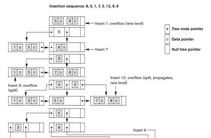
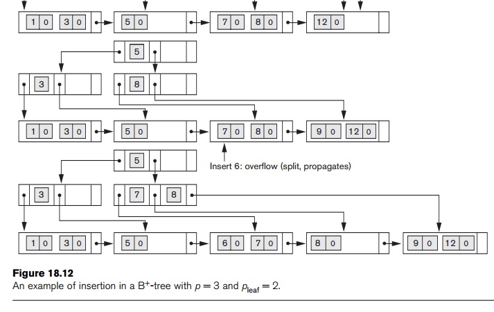
Figure 18.12 illustrates insertion of records in a B⁺-tree of order p = 3 and p_leaf = 2. First, we observe that the root is the only node in the tree, so it is also a leaf node. As soon as more than one level is created, the tree is divided into internal nodes and leaf nodes. Notice that every key value must exist at the leaf level, because all data pointers are at the leaf level. However, only some values exist in internal nodes to guide the search. Notice also that every value appearing in an internal node also appears as the rightmost value in the leaf level of the subtree pointed at by the tree pointer to the left of the value.

When a leaf node is full and a new entry is inserted there, the node overflows and

must be split. The first j = ((p_leaf + 1)/2) entries in the original node are kept there, and the remaining entries are moved to a new leaf node. The jth search value

is replicated in the parent internal node, and an extra pointer to the new node is created in the parent. These must be inserted in the parent node in their correct sequence. If the parent internal node is full, the new value will cause it to overflow also, so it must be split. The entries in the internal node up to P_j—the jth tree pointer after inserting the new value and pointer, where j = ((p + 1)/2) —are kept, while the jth search value is moved to the parent, not replicated. A new internal node will hold the entries from P_j+1 to the end of the entries in the node (see Algorithm 18.3). This splitting can propagate all the way up to create a new root node and hence a new level for the B⁺-tree.

Figure 18.13 illustrates deletion from a B⁺-tree. When an entry is deleted, it is always removed from the leaf level. If it happens to occur in an internal node, it must also be removed from there. In the latter case, the value to its left in the leaf node must replace it in the internal node because that value is now the rightmost entry in the subtree. Deletion may cause underflow by reducing the number of entries in the leaf node to below the minimum required. In this case, we try to find a sibling leaf node—a leaf node directly to the left or to the right of the node with underflow

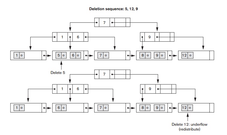
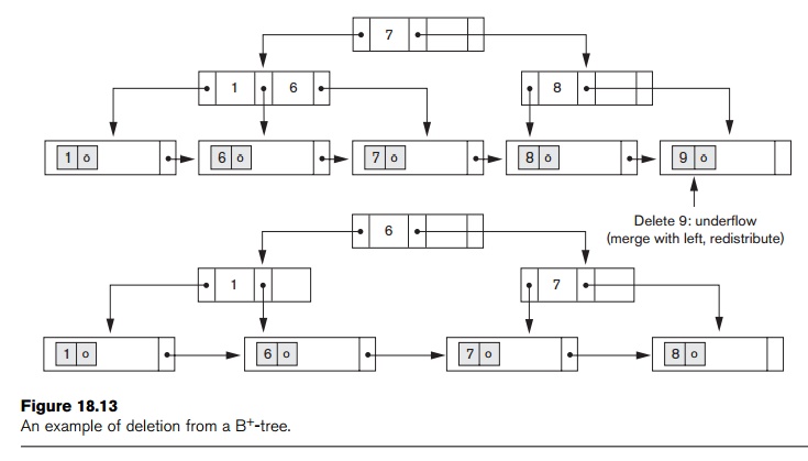
and redistribute the entries among the node and its sibling so that both are at least half full; otherwise, the node is merged with its siblings and the number of leaf nodes is reduced. A common method is to try to redistribute entries with the left sibling; if this is not possible, an attempt to redistribute with the right sibling is made. If this is also not possible, the three nodes are merged into two leaf nodes. In such a case, underflow may propagate to internal nodes because one fewer tree pointer and search value are needed. This can propagate and reduce the tree levels.

Notice that implementing the insertion and deletion algorithms may require parent and sibling pointers for each node, or the use of a stack as in Algorithm 18.3. Each node should also include the number of entries in it and its type (leaf or internal). Another alternative is to implement insertion and deletion as recursive procedures.

Variations of B-Trees and B⁺-Trees. To conclude this section, we briefly mention some variations of B-trees and B⁺-trees. In some cases, constraint 5 on the B-tree (or for the internal nodes of the B⁺–tree, except the root node), which requires each node to be at least half full, can be changed to require each node to be at least two-thirds full. In this case the B-tree has been called a B*-tree. In general, some systems allow the user to choose a fill factor between 0.5 and 1.0, where the latter means that the B-tree (index) nodes are to be completely full. It is also possible to specify two fill factors for a B⁺-tree: one for the leaf level and one for the internal nodes of the tree. When the index is first constructed, each node is filled up to approximately the fill factors specified. Some investigators have suggested relaxing the requirement that a node be half full, and instead allow a node to become completely empty before merging, to simplify the deletion algorithm. Simulation studies show that this does not waste too much additional space under randomly distributed insertions and deletions.