Indexes on Multiple Keys

Indexes on Multiple Keys

In our discussion so far, we have assumed that the primary or secondary keys on which files were accessed were single attributes (fields). In many retrieval and update requests, multiple attributes are involved. If a certain combination of attributes is used frequently, it is advantageous to set up an access structure to provide efficient access by a key value that is a combination of those attributes.

For example, consider an EMPLOYEE file containing attributes Dno (department number), Age, Street, City, Zip_code, Salary and Skill_code, with the key of Ssn (Social Security number). Consider the query: List the employees in department number 4 whose age is 59. Note that both Dno and Age are nonkey attributes, which means that a search value for either of these will point to multiple records. The following alter-native search strategies may be considered:

1.     Assuming Dno has an index, but Age does not, access the records having Dno = 4 using the index, and then select from among them those records that satisfy Age = 59.

2.    Alternately, if Age is indexed but Dno is not, access the records having Age = 59 using the index, and then select from among them those records that satisfy Dno = 4.

3.    If indexes have been created on both Dno and Age, both indexes may be used; each gives a set of records or a set of pointers (to blocks or records). An inter-section of these sets of records or pointers yields those records or pointers that satisfy both conditions.

All of these alternatives eventually give the correct result. However, if the set of records that meet each condition (Dno = 4 or Age = 59) individually are large, yet only a few records satisfy the combined condition, then none of the above is an efficient technique for the given search request. A number of possibilities exist that would treat the combination < Dno, Age> or < Age, Dno> as a search key made up of multiple attributes. We briefly outline these techniques in the following sections. We will refer to keys containing multiple attributes as composite keys.

1. Ordered Index on Multiple Attributes

All the discussion in this chapter so far still applies if we create an index on a search key field that is a combination of <Dno, Age>. The search key is a pair of values <4, 59> in the above example. In general, if an index is created on attributes <A₁, A₂, ..., A_n>, the search key values are tuples with n values: <v₁, v₂, ..., v_n>.

A lexicographic ordering of these tuple values establishes an order on this composite search key. For our example, all of the department keys for department number 3 precede those for department number 4. Thus <3, n> precedes <4, m> for any values of m and n. The ascending key order for keys with Dno = 4 would be <4, 18>, <4, 19>, <4, 20>, and so on. Lexicographic ordering works similarly to ordering of character strings. An index on a composite key of n attributes works similarly to any index discussed in this chapter so far.

2. Partitioned Hashing

Partitioned hashing is an extension of static external hashing (Section 17.8.2) that allows access on multiple keys. It is suitable only for equality comparisons; range queries are not supported. In partitioned hashing, for a key consisting of n components, the hash function is designed to produce a result with n separate hash addresses. The bucket address is a concatenation of these n addresses. It is then pos-sible to search for the required composite search key by looking up the appropriate buckets that match the parts of the address in which we are interested.

For example, consider the composite search key <Dno, Age>. If Dno and Age are hashed into a 3-bit and 5-bit address respectively, we get an 8-bit bucket address. Suppose that Dno = 4 has a hash address ‘100’ and Age = 59 has hash address ‘10101’. Then to search for the combined search value, Dno = 4 and Age = 59, one goes to bucket address 100 10101; just to search for all employees with Age = 59, all buckets (eight of them) will be searched whose addresses are ‘000 10101’, ‘001 10101’, ... and so on. An advantage of partitioned hashing is that it can be easily extended to any number of attributes. The bucket addresses can be designed so that high-order bits in the addresses correspond to more frequently accessed attributes. Additionally, no separate access structure needs to be maintained for the individual attributes. The main drawback of partitioned hashing is that it cannot handle range queries on any of the component attributes.

3. Grid Files

Another alternative is to organize the EMPLOYEE file as a grid file. If we want to access a file on two keys, say Dno and Age as in our example, we can construct a grid array with one linear scale (or dimension) for each of the search attributes. Figure 18.14 shows a grid array for the EMPLOYEE file with one linear scale for Dno and another for the Age attribute. The scales are made in a way as to achieve a uniform distribution of that attribute. Thus, in our example, we show that the linear scale for Dno has Dno = 1, 2 combined as one value 0 on the scale, while Dno = 5 corresponds to the value 2 on that scale. Similarly, Age is divided into its scale of 0 to 5 by grouping ages so as to distribute the employees uniformly by age. The grid array shown for this file has a total of 36 cells. Each cell points to some bucket address where the records corresponding to that cell are stored. Figure 18.14 also shows the assignment of cells to buckets (only partially).

Thus our request for Dno = 4 and Age = 59 maps into the cell (1, 5) corresponding to the grid array. The records for this combination will be found in the correspond-ing bucket. This method is particularly useful for range queries that would map into a set of cells corresponding to a group of values along the linear scales. If a range query corresponds to a match on the some of the grid cells, it can be processed by accessing exactly the buckets for those grid cells. For example, a query for Dno ≤ 5

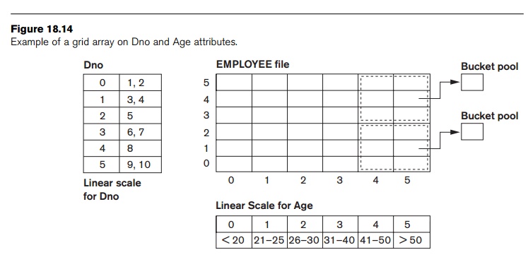
and Age > 40 refers to the data in the top bucket shown in Figure 18.14. The grid file concept can be applied to any number of search keys. For example, for n search keys, the grid array would have n dimensions. The grid array thus allows a partitioning of the file along the dimensions of the search key attributes and provides an access by combinations of values along those dimensions. Grid files perform well in terms of reduction in time for multiple key access. However, they represent a space overhead in terms of the grid array structure. Moreover, with dynamic files, a frequent reorganization of the file adds to the maintenance cost.