Mathematics for Cryptography

Mathematics for Cryptography

Encryption is a two-edged sword: We want to encrypt important information relatively easily, but we would like an attacker to have to work very hard to break an encryptionso hard that the attacker will stop trying to break the encryption and focus instead on a different method of attack (or, even better, a different potential victim).

To accomplish these goals, we try to force an interceptor to solve a hard problem, such as figuring out the algorithm that selected one of n! permutations of the original message or data. However, the interceptor may simply generate all possible permutations and scan them visually (or with some computer assistance), looking for probable text. Thus, the interceptor need not solve our hard problem. We noted in Chapter 2 the many ways this could happen. Indeed, the interceptor might solve the easier problem of determining which permutation was used in this instance. Remember that the attacker can use any approach that works. Thus, it behooves us as security specialists to make life difficult for the interceptor, no matter what method is used to break the encryption. In this section, we look particularly at how to embed the algorithm in a problem that is extremely difficult to solve. By that, we mean either that there is no conceivable way of determining the algorithm from the ciphertext or that it takes too long to reconstruct the plaintext to be worth the attacker's time.

Complexity

If the encryption algorithm is based on a problem that is known to be difficult to solve and for which the number of possible solutions is very large, then the attacker has a daunting if not impossible task. In this case, even with computer support, an exhaustive brute force solution is expected to be infeasible. Researchers in computer science and applied mathematics help us find these "hard problems" by studying and analyzing the inherent complexity of problems. Their goal is to say not only that a particular solution (or algorithm) is time consuming, but also that there simply is no easy solution. Much of the important work in this area was done in the early 1970s, under the general name of computational complexity. Thus, we begin our study of secure encryption systems by developing a foundation in problem complexity; we also introduce the mathematical concepts we need to understand the theory.

NP-Complete Problems

Cook [COO71] and Karp [KAR72] conducted an important investigation of problem complexity based on what are called NP-complete problems. The mathematics of the problems' complexity is daunting, so we present the notions intuitively, by studying three problems. Each of the problems is easy to state, not hard to understand, and straightforward to solve. Each also happens to be NP-complete. After we describe and discuss the problems, we develop the precise meaning of NP-completeness.

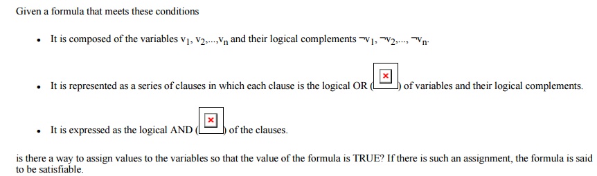
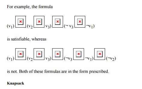
Satisfiability

Consider the problem of determining whether any given logical formula is satisfiable. That is, for a given formula, we want to know whether there is a way of assigning the values TRUE and FALSE to the variables so that the result of the formula is TRUE. Formally, the problem is presented as follows.

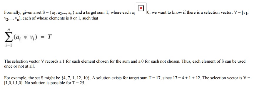
The name of the problem relates to placing items into a knapsack. Is there a way to select some of the items to be packed such that their "sum" (the amount of space they take up) exactly equals the knapsack capacity (the target)? We can express the problem as a case of adding integers. Given a set of nonnegative integers and a target, is there a subset of the integers whose sum equals the target?

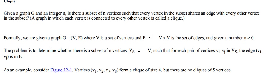
Characteristics of NP-Complete Problems

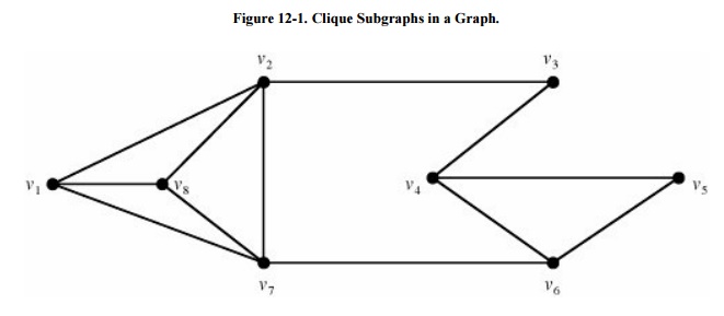
These three problems are reasonable representatives of the class of NP-complete problems. Notice that they share the following characteristics.

Each problem is solvable, and a relatively simple approach solves it (although the approach may be time consuming). For each of them, we can simply enumerate all the possibilities: all ways of assigning the logical values of n variables, all subsets of the set S, all subsets of n vertices in G. If there is a solution, it will appear in the enumeration of all possibilities; if there is no solution, testing all possibilities will demonstrate that.

   There are 2ⁿ cases to consider if we use the approach of enumerating all possibilities (where n depends on the problem). Each possibility can be tested in a relatively small amount of time, so the time to test all possibilities and answer yes or no is proportional to 2ⁿ.

   The problems are apparently unrelated, having come from logic, number theory, and graph theory, respectively.

   If it were possible to guess perfectly, we could solve each problem in relatively little time. For example, if someone could guess the correct assignment or the correct subset, we could simply verify that the formula had been satisfied or a correct sum had been determined, or a clique had been identified. The verification process could be done in time bounded by a polynomial function of the size of the problem.

The Classes P and NP

Let P be the collection of all problems for which there is a solution that runs in time bounded by a polynomial function of the size of the problem. For example, you can determine if an item is in a list in time proportional to the size of the list (simply by examining each element in the list to determine if it is the correct one), and you can sort all items in a list into ascending order in time bounded by the square of the number of elements in the list (using, for example, the well-known bubble sort algorithm.) There may also be faster solutions;

that is not important here. Both the searching problem and the sorting problem are in P, since they can be solved in time n and n², respectively.

For most problems, polynomial time algorithms reach the limit of feasible complexity. Any problem that could be solved in time n^{1,000,000,000} would be in P, even though for large values of n, the time to perform such an algorithm might be prohibitive. Notice also that we do not have to know an explicit algorithm; we just have to be able to say that such an algorithm exists.

By contrast, let NP be the set of all problems that can be solved in time bounded by a polynomial function of the size of the problem, assuming the ability to guess perfectly. (In the literature, this "guess function" is called an oracle or a nondeterministic Turing machine). The guessing is called nondeterminism.

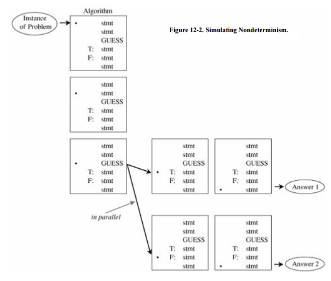
Of course, no one can guess perfectly. We simulate guessing by cloning an algorithm and applying one version of it to each possible outcome of the guess, as shown in Figure 12-2. Essentially, the idea is equivalent to a computer programming language in which IF statements could be replaced by GUESS statements: Instead of testing a known condition and branching depending on the outcome of the test, the GUESS statements would cause the program to fork, following two or more paths concurrently.

The ability to guess can be useful. For example, instead of deciding whether to assign the value TRUE or FALSE to variable v₁, the nondeterministic algorithm can proceed in two directions: one assuming TRUE had been assigned to v₁ and the other assuming FALSE. As the number of variables increases so does the number of possible paths to be pursued concurrently.

Certainly, every problem in P is also in NP, since the guess function does not have to be invoked. Also, a class, EXP, consists of problems  for which a deterministic solution exists in exponential time, cn for some constant c. As noted earlier, every NP-complete problem has such a solution. Every problem in NP is also in EXP, so P NP EXP.  

The Meaning of NP-Completeness

Cook [COO71] showed that the satisfiability problem is NP-complete, meaning that it can represent the entire class NP. His important conclusion was that if there is a deterministic, polynomial time algorithm (one without guesses) for the satisfiability problem, then there is a deterministic, polynomial time algorithm for every problem in NP; that is, P = NP.

Karp [KAR72] extended Cook's result by identifying a number of other problems, all of which shared the property that if any one of them could be solved in a deterministic manner in polynomial time, then all of them could. The knapsack and clique problems were identified by Karp as having this property. The results of Cook and Karp included the converse: If for even one of these problems (or any NP-complete problem) it could be shown that there was no deterministic algorithm that ran in polynomial time, then no deterministic algorithm could exist for any of them.

In discussing problem complexity, we must take care to distinguish between a problem and an instance of a problem. An instance is a specific case: one formula, one specific graph, or one particular set S. Certain simple graphs or simple formulas may have solutions that are easy and fast to identify. A problem is more general; it is the description of all instances of a given type. For example, the formal statements of the satisfiability, knapsack, and clique questions are statements of problems, since they tell what each specific instance of that problem must look like. Solving a problem requires finding one general algorithm that solves every instance of that problem.

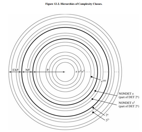
Essentially the problem space (that is, the classification of all problems) looks like Figure 12-3. There are problems known to be solvable deterministically in polynomial time (P), and there are problems known not to have a polynomial time solution (EXP and beyond), so  EXP and P EXP, meaning P EXP and we can also show NP EXP. The class NP fits somewhere between P and EXP: P NP EXP. It may be that P = NP, or that P NP.

The significance of Cook's result is that NP-complete problems have been studied for a long time by many different groups of peoplelogicians, operations research specialists, electrical engineers, number theorists, operating systems specialists, and communications engineers. If there were a practical (polynomial time) solution to any one of these problems, we would hope that someone would have found it by now. Currently, several hundred problems have been identified as NP-complete. (Garey and Johnson [GAR79] catalog many NP-complete problems.) The more problems in the list, the stronger the reason to believe that there is no simple (polynomial time) solution to any (all) of them.

NP-Completeness and Cryptography

Hard-to-solve problems are fundamental to cryptography. Basing an encryption algorithm on one of these hard problems would seem to be a way to require the interceptor to do a prodigious amount of work to break the encryption. Unfortunately, this line of reasoning has four fallacies.

   An NP-complete problem does not guarantee that there is no solution easier than exponential; it merely indicates that we are unlikely to find an easier solution. This distinction means that the basis of the difficulty in cracking an encryption algorithm might deteriorate if someone should show that P = NP. This is the least serious of the fallacies.

Every NP-complete problem has a deterministic exponential time solution, that is, one that runs in time proportional to 2ⁿ. For small values of n, 2ⁿ is not large, and so the work of the interceptor using a brute force attack may not be prohibitive. We can get around this difficulty by selecting the algorithm so that the instance of the problem is very large; that is, if n is large, 2ⁿ will be appropriately deterring.

   Continuing advances in hardware make problems of larger and larger size tractable. For example, parallel processing machines are now being designed with a finite but large number of processors running together. With a GUESS program, two processors could simultaneously follow the paths from a GUESS point. A large number of processors could complete certain nondeterministic programs in deterministic mode in polynomial time. However, we can select the problem's setting so that the value of n is large enough to require an unreasonable number of parallel processors. (What seems unreasonable now may become reasonable in the future, so we need to select n with plenty of room for growth.)

   Even if an encryption algorithm is based on a hard problem, the interceptor does not always have to solve the hard problem to crack the encryption. In fact, to be useful for encryption, these problems must have a secret, easy solution. An interceptor may look for the easy way instead of trying to solve a hard underlying problem. We study an example of this type of exposure later in this chapter when we investigate the MerkleHellman knapsack algorithm.

Other Inherently Hard Problems

Another source of inherently difficult problems is number theory. These problems are appealing because they relate to numeric computation, so their implementation is natural on computers. Since number theory problems have been the subject of much recent research, the lack of easy solutions inspires confidence in their basic complexity. Most of the number theory problems are not NP-complete, but the known algorithms are very time consuming nevertheless.

Two such problems that form the basis for secure encryption systems are computation in Galois fields and factoring large numbers. In the next section we review topics in algebra and number theory that enable us to understand and use these problems.

Properties of Arithmetic

We begin with properties of multiplication and division on integers. In particular, we investigate prime numbers, divisors, and factoring since these topics have major implications in building secure encryption algorithms. We also study a restricted arithmetic system, called a "field." The fields we consider are finite and have convenient properties that make them very useful for representing cryptosystems.

Unless we explicitly state otherwise, this section considers only arithmetic on integers. Also, unless explicitly stated otherwise, we use conventional, not mod n, arithmetic in this section.

Inverses

Let • be an operation on numbers. For example, • might be + (addition) or * (multiplication) . A number i is called an identity for • if x • i = x and i • x = x for every number x. For example, 0 is an identity for +, since x + 0 = x and 0 + x = x. Similarly, 1 is an identity for *.

Let i be an identity for •. The number b is called the inverse of a under • if a • b = i and b • a = i. An identity holds for an entire operation; an inverse is specific to a single number. The identity element is always its own inverse, since i • i = i. The inverse of an element a is

sometimes denoted a^-1.

Using addition on integers as an example operation, we observe that the inverse of any element a is (- a), since a + (-a) = 0. When we consider the operation of multiplication on the rational numbers, the inverse of any element a (except 0) is 1/a, since a * (1/a) = 1. However, under the operation of multiplication on the integers, there are no inverses (except 1). Consider, for example, the integer 2. There is no other integer b such that 2 * b = 1. The positive integers under the operation + have no inverses either.

Primes

To say that one number divides another, or that the second is divisible by the first, means that the remainder of dividing the second by the first is 0. Thus, we say that 2 divides 10, since 10/2 = 5 with remainder 0. However, 3 does not divide 10, since 10/3 = 3 with remainder 1. Also, the fact that 2 divides 10 does not necessarily mean that 10 divides 2; 2/10 = 0 with remainder 2.

A prime number is any number greater than 1 that is divisible (with remainder 0) only by itself and 1.^[1] For example, 2, 3, 5, 7, 11, and 13 are primes, whereas 4 (2 * 2), 6 (2 * 3), 8 (2 * 2 * 2), and 9 (3 * 3) are not. A number that is not a prime is a composite.

^[1] We disregard -1 as a factor, since (-1) * (-1) = 1.

Greatest Common Divisor

The greatest common divisor of two numbers, a and b, is the largest integer that divides both a and b. The greatest common divisor is often written gcd(a, b). For example, gcd(15, 10) = 5 since 5 divides both 10 and 15, and nothing larger than 5 does. If p is a prime, for any number q < p, gcd(p, q) = 1. Clearly, gcd(a, b) = gcd(b, a).

Euclidean Algorithm

The Euclidean algorithm is a procedure for computing the greatest common divisor of two numbers. This algorithm exploits the fact that if x divides a and b, x also divides a - (k * b) for every k. To understand why, if x divides both a and b, then a = x * a₁ and b = x * b₁. But then,

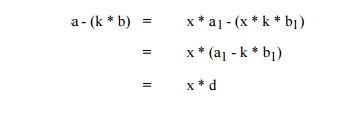
so that x divides (is a factor of) a - (k * b).

This result leads to a simple algorithm for computing the greatest common denominator of two integers. Suppose we want to find x, the gcd of a and b, where a > b.

Rewrite a as

a = m * b + r

where 0<  r < b. (In other words, compute m = a/b with remainder r.) If x = gcd(a,b), x divides a, x divides b, and x divides r. But gcd (a, b) = gcd(b, r) and a > b > r > 0. Therefore, we can simplify the search for gcd by working with b and r instead of a and b: b = m' * r + r'

where m' = b/r with remainder r'. This result leads to a simple iterative algorithm, which terminates when a remainder 0 is found.

Example

For example, to compute gcd(3615807, 2763323), we take the following steps.

3,615,807 = (1) * 2,763,323 + 852,484

2,763,323 = (3) * 852,484 + 205,871

852,484  = (4) * 205,871 + 29,000

205,871  = (7) * 29,000+2,871

29,000   = (10) * 2,871 + 290

2,871    = (9) * 290 + 261

290     = (1) * 261 + 29

261     =(9) * 29 + 0

Thus, gcd(3615807, 2763323) = 29.

Modular Arithmetic

Modular arithmetic offers us a way to confine results to a particular range, just as the hours on a clock face confine us to reporting time relative to 12 or 24. We have seen in earlier chapters how, in some cryptographic applications, we want to perform some arithmetic

operations on a plaintext character and guarantee that the result will be another character. Modular arithmetic enables us to do this; the results stay in the underlying range of numbers. An even more useful property is that the operations +, -, and * can be applied before or after the modulus is taken, with similar results.

Recall that a modulus applied to a nonnegative integer means remainder after division, so that 11 mod 3 = 2 since 11/3 = 3 with remainder 2. If a mod n = b then

a = c * n + b

for some integer c. Two different integers can have the same modulus: 11 mod 3 = 2 and 5 mod 3 = 2. Any two integers are equivalent under modulus n if their results mod n are equal. This property is denoted

x n y if and only if (x mod n) = (y mod n)

x n y if and only if (x - y) = k * n for some k 

In the following sections, unless we use parentheses to indicate otherwise, a modulus applies to a complete expression. Thus, you should interpret a + b mod n as (a + b) mod n, not a + (b mod n).

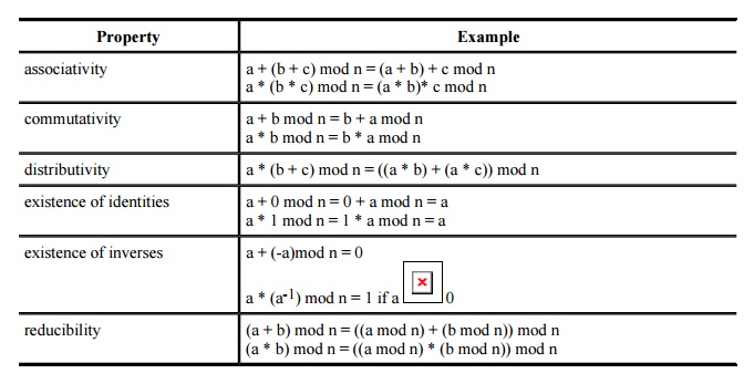
Properties of Modular Arithmetic

Modular arithmetic on the nonnegative integers forms a construct called a commutative ring with operations + and * (addition and multiplication). Furthermore, if every number other than 0 has an inverse under *, the group is called a Galois field. All rings have the properties of associativity and distributivity; commutative rings, as their name implies, also have commutativity. Inverses under multiplication produce a Galois field. In particular, the integers mod a prime n are a Galois field. The properties of this arithmetic system are listed here.

Example

As an example, consider the field of integers mod 5 shown in the tables below. These tables illustrate how to compute the sum or product of any two integers mod 5. However, the reducibility rule gives a method that you may find easier to use. To compute the sum or product of two integers mod 5, we compute the regular sum or product and then reduce this result by subtracting 5 until the result is between 0 and 4. Alternatively, we divide by 5 and keep only the remainder after division.

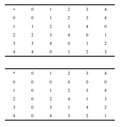
For example, let us compute 3 + 4 mod 5. Since 3 + 4 = 7 and 7 - 5 = 2, we can conclude that 3 + 4 mod 5 = 2. This fact is confirmed by the table. Similarly, to compute 4 * 4 mod 5, we compute 4 * 4 = 16. We can compute 16 - 5 = 11 - 5 = 6 - 5 = 1, or we can compute 16/5 = 3 with remainder 1. Either of these two approaches shows that 4 * 4 mod 5 = 1, as noted in the table. Since constructing the tables shown is difficult for large values of the modulus, the remainder technique is especially helpful.

Computing Inverses

In the ordinary system of multiplication on rational numbers, the inverse of any nonzero number a is 1/a, since a * (1/a) = 1. Finding inverses is not quite so easy in the finite fields just described. In this section we learn how to determine the multiplicative inverse of any element.

The inverse of any element a is that element b such that a * b = 1. The multiplicative inverse of a can be written a^-1. Looking at the table for multiplication mod 5, we find that the inverse of 1 is 1, the inverse of 2 is 3 and, since multiplication is commutative, the inverse of 3 is also 2; finally, the inverse of 4 is 4. These values came from inspection, not from any systematic algorithm.

To perform one of the secure encryptions, we need a procedure for finding the inverse mod n of any element, even for very large values of

n. An algorithm to determine a^-1 directly is likely to be faster than a table search, especially for large values of n. Also, although there is a pattern to the elements in the table, it is not easy to generate the elements of a particular row, looking for a 1 each time we need an inverse. Fortunately, we have an algorithm that is reasonably simple to compute.

Fermat's Theorem

In number theory, Fermat's theorem states that for any prime p and any element a < p,

a^p mod p = a

or

a^p-1 mod p = 1

This result leads to the inverses we want. For a prime p and an element a < p, the inverse of a is that element x such that

ax mod p = 1

Combining the last two equations, we obtain

ax mod p = 1 = a^p-1 mod p

so that

x = a^p-2 mod p

This method is not a complete method for computing inverses, in that it works only for a prime p and an element a < p.

Example

We can use this formula to determine the inverse of 3 mod 5:

                  3³ mod 5

                 27 mod 5

                 2

as we determined earlier from the multiplication table.

Algorithm for Computing Inverses

Another method to compute inverses is shown in the following algorithm. This algorithm, adapted from [KNU73], is a fast approach that uses Euclid's algorithm for finding the greatest common divisor.

{**Compute x = a^-1 mod n given a and n **}

We use these mathematical results in the next sections as we examine two encryption systems based on arithmetic in finite fields.