Hermite curve

Hermite curve

A Hermite curve is a spline where every piece is a third degree polynomial defined in Hermite form: that is, by its values and initial derivatives at the end points of the equivalent domain interval. Cubic Hermite splines are normally used for interpolation of numeric values defined at certain dispute values x1,x2,x3, …..xn,to achieve a smooth continuous function. The data should have the preferred function value and derivative at each Xk. The Hermite formula is used to every interval (Xk,

Xk+1) individually. The resulting spline become continuous and will have first derivative.

Cubic polynomial splines are specially used in computer geometric modeling to attain curves that pass via defined points of the plane in 3D space. In these purposes, each coordinate of the plane is individually interpolated by a cubic spline function of a divided parameter‘t’.

Cubic splines can be completed to functions of different parameters, in several ways. Bicubic splines are frequently used to interpolate data on a common rectangular grid, such as pixel values in a digital picture. Bicubic surface patches, described by three bicubic splines, are an necessary tool in computer graphics. Hermite curves are simple to calculate but also more powerful. They are used to well interpolate between key points.

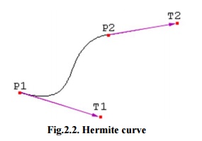
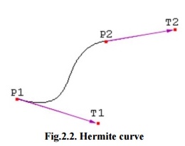
Fig.2.2. Hermite curve

The following vectors needs to compute a Hermite curve:

·        P1: the start point of the Hermite curve

·        T1: the tangent to the start point

·        P2: the endpoint of the Hermite curve

·        T2: the tangent to the endpoint

These four vectors are basically multiplied with four Hermite basis functions h1(s), h2(s), h3(s) and,h4(s) and added together.

h1(s) = 2s3 - 3s2 + 1 h2(s) = -2s3 + 3s2

h3(s) = s3 - 2s2 + s h4(s) = s3 - s2

Figure 2.3 shows the functions of Hermite Curve of the 4 functions (from left to right: h1, h2, h3, h4).

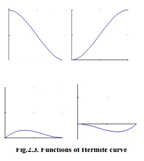
Fig.2.3. Functions of Hermite curve

A closer view at functions ‘h1’and ‘h2’,the result shows that function ‘h1’starts at one and goes slowly to zero and function ‘h2’starts at zero and goes slowly to one.

At the moment, multiply the start point with function ‘h1’and the endpoint with function ‘h2’. Let s varies from zero to one to interpolate between start and endpoint of Hermite Curve. Function

‘h3’and function ‘h4’are used to the tangents in the similar way. They make confident that the Hermite curve bends in the desired direction at the start and endpoint.