Bezier curves

Bezier curve

Bezier curves are extensively applied in CAD to model smooth curves. As the curve is totally limited in the convex hull of its control points P0, P1,P2 & P3, the points can be graphically represented and applied to manipulate the curve logically. The control points P0 and P3 of the polygon lie on the curve (Fig.2.4.). The other two vertices described the order, derivatives and curve shape. The Bezier curve is commonly tangent to first and last vertices.

Cubic Bezier curves and Quadratic Bezier curves are very common. Higher degree Bezier curves are highly computational to evaluate. When more complex shapes are required, Bezier curves in low order are patched together to produce a composite Bezier curve. A composite Bezier curve is usually described to as a ‘path’in vector graphics standards and programs. For smoothness assurance, the control point at which two curves meet should be on the line between the two control points on both sides.

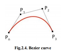
Fig.2.4. Bezier curve

A general adaptive method is recursive subdivision, in which a curve's control points are verified to view if the curve approximates a line segment to within a low tolerance. If not, the curve is further divided parametrically into two segments, 0 ≤t ≤0.5 and 0.5 ≤ ≤t1, and the same process is used recursively to each half. There are future promote differencing techniques, but more care must be taken to analyze error transmission.

Analytical methods where a Bezier is intersected with every scan line engage finding roots of cubic polynomials and having with multiple roots, so they are not often applied in practice. A Bezier curve is described by a set of control points P0 through Pn, where ‘n’is order of curve. The initial and end control points are commonly the end points of the curve; but, the intermediate control points normally do not lie on the curve.

(i)                Linear Bezier curves

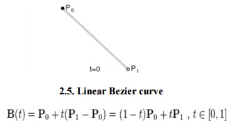
2.5. Linear Bezier curve

As shown in the figure 2.5, the given points P0 and P1, a linear Bezier curve is merely a straight line between those two points. The Bezier curve is represented by And it is similar to linear interpolation.

(ii) Quadratic Bezier curves

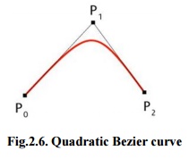
Fig.2.6. Quadratic Bezier curve

As shown in the figure 2.6, a quadratic Bezier curve is the path defined by the function B(t), given points P0, P1, and P2,

This can be interpreted as the linear interpolate of respective points on the linear Bezier curves from P0 to P1 and from P1 to P2 respectively. Reshuffle the preceding equation gives:

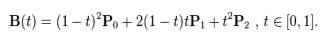
The derivative of the Bezier curve with respect to the value ‘t’is

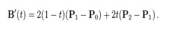
From  which  it  can  be  finished  that  the  tangents  to  the  curve  at P0  and P2  intersect  at P1.  While

‘t’increases from zero to one, the curve departs from P0 in the direction of P1, then turns to land at P2 from the direction of P1.

The following equation is a second derivative of the Bezier curve with respect to ‘t’:

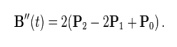
A quadratic Bezier curve is represent a  parabolic segment. Since a parabola curve is a conic section, a few sources refer to quadratic Beziers as ‘conic arcs’.

(iii) Cubic Bezier curves

As shown in figure 2.7, four control points P0, P1, P2 and P3 in the higher-dimensional space describe as a Cubic Bezier curve. The curve begins at P0 going on the way to P1 and reaches at P3 coming from the direction of P2. Typically, it will not pass through control points P1 / P2, these points are only there to give directional data. The distance between P0 and P1 determines ‘how fast’and ‘how far’the curve travels towards P1 before turning towards P2.

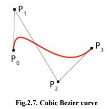
Fig.2.7. Cubic Bezier curve

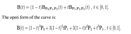
The function B Pi, Pj, Pk (t) for the quadratic Bezier curve written by points Pi, Pj, and Pk, the cubic Bezier curve can be described as a linear blending of two quadratic Bezier curves:

For several choices of P1  and P2  the Bezier curve may meet itself.

Any sequence of any four dissimilar points can be changed to a cubic Bezier curve that goes via all four points in order. Given the beginning and ending point of a few cubic Bezier curve, and the points beside the curve equivalent to t = 1/3 and t = 2/3, the control points for the original Bezier curve can be improved.

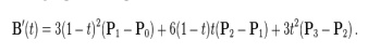
The following equation represent first derivative of the cubic Bezier curve with respect to t:

The following equation represent second derivative of the Bezier curve with respect to t:

1. Properties Bezier curve

·       The Bezier curve starts at P0  and ends at Pn; this is known as ‘endpoint interpolation’property.

·       The Bezier curve is a straight line when all the control points of a cure are collinear.

·       The beginning of the Bezier curve is tangent to the first portion of the Bezier polygon.

·       A Bezier curve can be divided at any point into two sub curves, each of which is also a Bezier curve.

·       A few curves that look like simple, such as the circle, cannot be expressed accurately by a Bezier; via four piece cubic Bezier curve can similar a circle, with a maximum radial error of less than one part in a thousand (Fig.2.8).

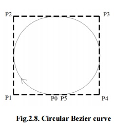
Fig.2.8. Circular Bezier curve

·       Each quadratic Bezier curve is become a cubic Bezier curve, and more commonly, each degree ‘n’Bezier curve is also a degree ‘m’curve for any m > n.

Bezier curves have the different diminishing property. A Bezier curves does not ‘ripple’more than the polygon of its control points, and may actually ‘ripple’lss than that.

·       Bezier curve is similar with respect to t and (1-t). This represents that the sequence of control points defining the curve can be changes without modify of the curve shape.

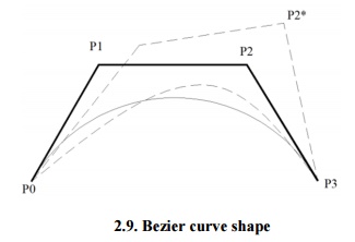
·       Bezier curve shape can be edited by either modifying one or more vertices of its polygon or by keeping the polygon unchanged or simplifying multiple coincident points at a vertex (Fig .2.19).

2. Construction of Bezier curves

(i) Linear curves:

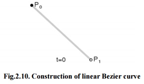
Fig.2.10. Construction of linear Bezier curve

The figure 2.10 shows the function for a linear Bezier curve can be via of as describing how far B(t) is from P0 to P1 with respect to ‘t’. When t equals to 0.25, B(t) is one quarter of the way from point P0 to P1. As ‘t’varies from 0 to 1, B(t) shows a straight line from P0 to P1.

(ii) Quadratic curves

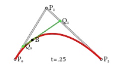
Fig.2.11. Construction of linear Quadratic curve

As  shown  in  figure  2.11,  a  quadratic  Bezier  curves  one  can  develop  by  intermediate

points Q0 and Q1  such that as ‘t’varies from 0 to 1:

·       Point Q0 (t) modifying from P0  to P1  and expresses a linear Bezier curve.

·       Point Q1 (t) modifying from P1  to P2  and expresses a linear Bezier curve.

·       Point B (t) is interpolated linearly between Q0(t) to Q1(t) and expresses a quadratic Bezier curve.

(iii) Higher-order curves

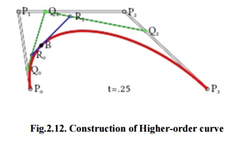
Fig.2.12. Construction of Higher-order curve

As shown in figure 2.12, a higher-order curves one requires correspondingly higher intermediate points. For create cubic curves, intermediate points Q0, Q1, and Q2 that express as linear

Bezier curves, and points R0  and R1  that express as quadratic Bezier curves.

3. Rational Bezier curve

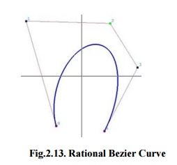
Fig.2.13. Rational Bezier Curve

The rational Bezier curve includes variable weights (w) to provide closer approximations to arbitrary shapes. For Rational Bezier Curve, the numerator is a weighted Bernstein form Bezier and the denominator is a weighted sum of Bernstein polynomials. Rational Bezier curves can be used to signify segments of conic sections accurately, including circular arcs (Fig.2.13).