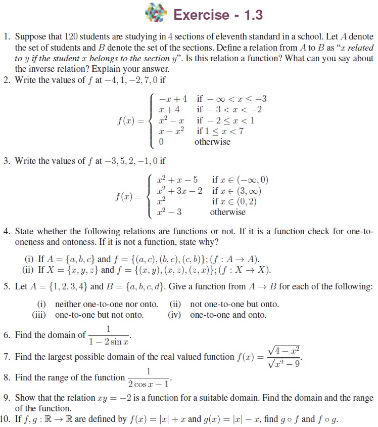
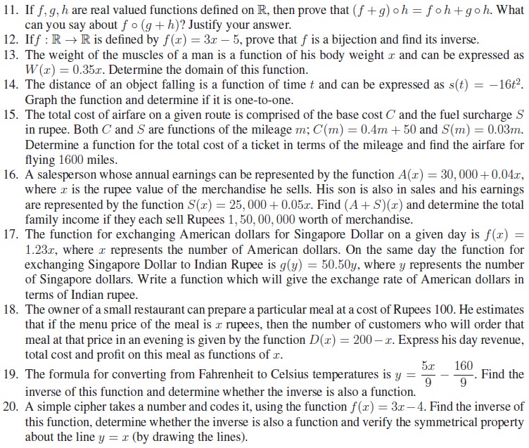
Functions

Functions

Suppose that a particle is moving in the space. We assume the physical particle as a point. As time varies, the particle changes its position. Mathematically at any time the point occupies a position in the three dimensional space R3. Let us assume that the time varies from 0 to 1. So the movement or functioning of the particle decides the position of the particle at any given time t between 0 and 1. In other words, for each t ∈ [0, 1], the functioning of the particle gives a point in R3. Let us denote the position of the particle at time t as f(t).

Let us see another simple example. We know that the equation 2x−y = 0 describes a straight line. Here whenever x assumes a value, y assumes some value accordingly. The movement or functioning of y is decided by that of x. Let us denote y by f(x). We may see many situation like this in nature. In the study of natural phenomena, we find that it is necessary to consider the variation of one quantity depending on the variation of another.

The relation of the time and the position of the particle, the relation of a point in the x-axis to a point in the y-axis and many more such relations are studied for a very long period in the name function. Before Cantor, the term function is defined as a rule which associates a variable with another variable. After the development of the concept of sets, a function is defined as a rule that associates for every element in a set A, a unique element in a set B. However the terms rule and associate are not properly defined mathematical terminologies. In modern mathematics every term we use has to be defined properly. So a definition for function is given using relations.

Suppose that we want to discuss a test written by a set of students. We shall see this as a relation. Let A be the set of students appeared for an examination and let B = {0, 1, 2, 3, . . . 100} be the set of possible marks. We define a relation R as follows:

A student a is related to a mark b if a got b marks in the test.

We observe the following from this example:

·        Every student got a mark. In other words, for every a ∈ A, there is an element b ∈ B such that (a, b) ∈ R.

·        A student cannot get two different marks in any test. In other words, for every a ∈ A, there is definitely only one b ∈ B such that (a, b) ∈ R. This can be restated in a different way: If (a, b), (a, c) ∈ R then b = c.

Relations having the above two properties form a very important class of relations, called functions.

Let us now have a rigorous definition of a function through relations.

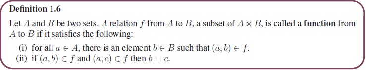
That is, a function is a relation in which each element in the domain is mapped to exactly one element in the range.

A is called the domain of f and B is called the co-domain of f. If (a, b) is in f, then we write f(a) = b; the element b is called the image of a and the element a is called a pre-image of b and f(a) is known as the value of f at a. The set {b : (a, b) ∈ f for some a ∈ A} is called the range of the function. If B is a subset of R, then we say that the function is a real-valued function.

Two functions f and g are said to be equal functions if their domains are same and f(a) = g(a) for all a in the domain.

If f is a function with domain A and co-domain B, we write f : A → B (Read this asf is from A to B or f be a function from A to B). We also say that f maps A into B. If f(a) = b, then we say f maps a to b or a is mapped onto b by f, and so on.

The range of a function is the collection of all elements in the co-domain which have pre-images. Clearly the range of a function is a subset of the co-domain. Further the first condition says that every element in the domain must have an image; this is the reason for defining the domain of a relation R from a set A to a set B as the set of all elements of A having images and not as A. The second condition says that an element in the domain cannot have two or more images.

Naturally one may have the following doubts:

·        In the definition, why we use the definite article “the” for image of a and the indefinite article “a” for pre-image of b?

·        We have a condition stating that every element in the domain must have an image; is there any condition like “every element in the co-domain must have a pre-image”? If not, why?

·        We have a condition stating that an element in the domain cannot have two or more images; is there any condition like “an element in the co-domain cannot have two or more pre-images”? If not, why?

As an element in the domain has exactly one image and an element in the co-domain can have more than one pre-image according to the definition, we use the definite article “the” for image of a and the indefinite article “a” for pre-image of b. There are no conditions as asked in the other two questions; the reason behind it can be understood from the problem of students’ mark we considered above.

We observe that every function is a relation but a relation need not be a function.

Let f = {(a, 1), (b, 2), (c, 2), (d, 4)}.

Is f a function? This is a function from the set {a, b, c, d} to {1, 2, 4}. This is not a function from {a, b, c, d, e} to {1, 2, 3, 4} because e has no image. This is not a function from {a, b, c, d} to {1, 2, 3, 5} because the image of d is not in the co-domain; f is not a subset of {a, b, c, d}×{1, 2, 3, 5}. So whenever we consider a function the domain and the co-domain must be stated explicitly.

The relation discussed in Illustration 1.1 is a function with domain {L, E, T, U, S, W, I, N} and co-domain {O, H, W, X, V, Z, L, Q}. The relation discussed in Illustration 1.3 is again a function with domain {a, b, . . . , z} and the co-domain {1, 2, 3, . . . , 26}.

In Illustration 1.2, we discussed three relations, namely

(i) y = 2x

 (ii) y = x2

(iii) y2 = x.

Clearly (i) and (ii) are functions whereas (iii) is not a function, if the domain and the co-domain are R. In (iii) for the same x, we have two y values which contradict the definition of the function. But if we split into two relations, that is, y = √x and y = −√x then both become functions with same domain non-negative real numbers and the co-domains [0, ∞) and (−∞, 0] respectively.

1. Ways of Representing Functions

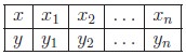
(a) Tabular Representation of a Function

When the elements of the domain are listed like x1, x2, x3 . . . xn, we can use this tabular form.Here, the values of the arguments x1, x2, x3 . . . xn and the corresponding values of the function y1, y2, y3 . . . yn are written out in a definite order.

(b) Graphical Representation of a Function

When the domain and the co-domain are subsets of R, many functions can be represented using a graph with x-axis representing the domain and y-axis representing the co-domain in the (x, y)-plane.

We note that the first and second figures in Illustration 1.2 represent the functions f(x) = 2x and f(x) = x2 respectively. Usually the variable x is treated as independent variable and y as a dependent variable. The variable x is called the argument and f(x) is called the value.

(c) Analytical Representation of a Function

If the functional relation y = f(x) is such that f denotes an analytical expression, we say that the function y of x is represented or defined analytically. Some examples of analytical expressions are

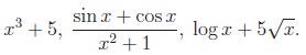
That is, a series of symbols denoting certain mathematical operations that are performed in a definite sequence on numbers, letters which designate constants or variable quantities.

Examples of functions defined analytically are

One of the usages of writing functions analytically is finding domains naturally. That is, the set of values of x for which the analytical expressions on the right-hand side has a definite value is the natural domain of definition of a function represented analytically.

Thus, the natural domain of the function,

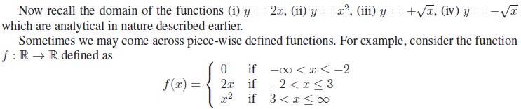
Depending upon the value of x, we have to select the formula to be used to find the value of f at any point x. To find the value off at any real number, first we have to find to which interval x belongs to; then using the corresponding formula we can find the value of f at that point. To find f(6) we know 3 ≤ 6 ≤ ∞ (or 6 ∈ [3, ∞)); so we use the formula f(x) = x2 and find f(6) = 36. Similarly f(−1) = −2, f(−5) = 0 and so on.

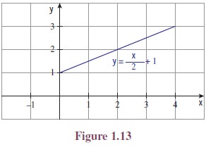
If the function is defined from R or a subset of R then we can draw the graph of the function. For example, if f : [0, 4] → R is defined by f(x) = x/2 + 1, then we can plot the points (x, x/2 + 1) for all ∈ [0, 4]. Then we will get a straight line segment joining (0, 1) and (4, 3). (See Figure 1.13)

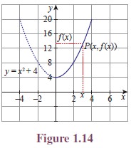
Consider another function f(x) = x2 + 4, x ≥ 0. The function will be given by its graph. (See Figure 1.14)

Let x be a point in the domain. Let us draw a vertical line through the point x. Let it meet the curve at P . The point at which the horizontal line drawn through P meets the y-axis is f(x). Similarly using horizontal lines through a point y in the co-domain, we can find the pre-images of y.

Can we say that any curve drawn on the plane be considered as a function from a subset of R to R? No, we cannot. There is a simple test to find this.

Vertical Line Test

As we noted earlier, the vertical line through any point x in the domain meets the curve at some point, then the y-coordinate of the point is f(x). If the vertical line through a point x in the domain meets the curve at more than one point, we will get more than one value for f(x) for one x. This is not allowed in a function. Further, if the vertical line through a point x in the domain does not meet the curve, then there will be no image for x; this is also not possible in a function. So we can say,

“if the vertical line through a point x in the domain meets the curve at more than one point or does not meet the curve, then the curve will not represent a function”.

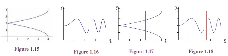
The curve indicated in Figure 1.15 does not represent a function from [0, 4] to R because a vertical line meets the curve at more than one point (See Figure 1.17). The curve indicated in Figure 1.16 does not represent a function from [0, 4] to R because a vertical line drawn through x = 2.5 in [0, 4] does not meet the curve (See Figure 1.18).

Testing whether a given curve represents a function or not by drawing vertical lines is called vertical line test or simply vertical test.

The third curve y2 = x in Illustration 1.2 fails in the vertical line test and hence it is not a function from R to R.

2. Some Elementary Functions

Some frequently used functions are known by names. Let us list some of them.

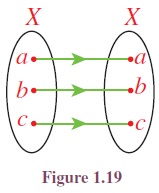
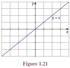
(i) Let X be any non-empty set. The function f : X → X defined by f(x) = x for all x ∈ X is called the identity function on X (See Figure 1.19). It is denoted by IX or I.

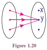
(ii) Let X and Y be two sets. Let c be a fixed element of Y . The function f : X → Y defined by f(x) = c for all x ∈ X is called a constant function (See Figure 1.20).

The value of a constant function is same for all values of x throughout the domain.

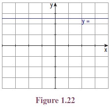
If X and Y are R, then the graph of the identity function and a constant function are as in Figures 1.21 and 1.22. If X is any set, then the constant function defined by f(x) = 0 for all x is called the zero function. So zero function is a particular case of constant function.

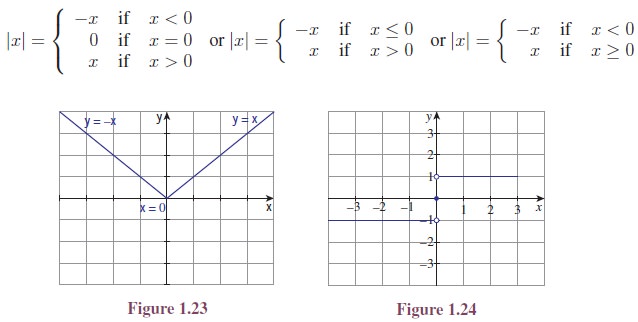
(iii) The function f : R → R defined by f(x) = |x|, where |x| is the modulus or absolute value of x, is called the modulus function or absolute value function. (See Figure 1.23.)

Let us recall that |x| is defined as

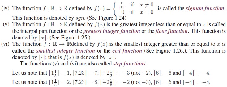
One may note the relations among the names of these functions, the symbols denoting the functions and the commonly used words ceiling and floor of a room and their graphs are given in Figures 1.25 and 1.26.

3. Types of Functions

Though functions can be classified into various types according to the need, we are going to concentrate on two basic types: one-to-one functions and onto functions.

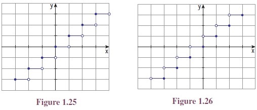
Let us look at the two simple functions given in Figure 1.27 and Figure 1.28. In the first function two elements of the domain, b and c, are mapped into the same element y, whereas it is not the case in the Figure 1.28. Functions like the second one are examples of one-to-one functions.

Let us look at the two functions given in Figures 1.28 and 1.29. In Figure 1.28 the element z in the co-domain has no pre-image, whereas it is not the case in Figure 1.29. Functions like in Figure 1.29 are example of onto functions. Now we define one-to-one and onto functions.

Another name for one-to-one function is injective function; onto function is surjective function. A function f : A → B is said to be bijective if it is both one-to-one and onto.

To prove a function f : A → B to be one-to-one, it is enough to prove any one of the following:

if x ¹ y, then f(x) ¹ f(y), or equivalently if f(x) = f(y), then x = y.

It is easy to observe that every identity function is one-to-one function as well as onto. A constant function is not onto unless the co-domain contains only one element. The following statements are some important simple results.

Let A and B be two sets with m and n elements.

i.            There is no one-to-one function from A to B if m > n.

ii.            If there is an one-to-one function from A to B, then m ≤ n.

iii.            There is no onto function from A to B if m < n.

iv.            If there is an onto function from A to B, then m ≥ n.

v.            There is a bijection from A to B, if and only if, m = n.

vi.            There is no bijection from A to B if and only if, m != n.

Now, we recall Illustration 1.1. In this illustration the function f : C → D is defined by

f(L) = O, f(E) = H, f(T ) = W, f(U) = X, f(S) = V, f(W ) = Z, f(I) = L, f(N) = Q

where C = {L, E, T, U, S, W, I, N} and D = {O, H, W, X, V, Z, L, Q}, is an one-to-one and onto function.

In Illustration 1.3, the function f : A → N is defined by f(a) = 1, f(b) = 2, . . . , f(z) = 26, where A = {a, b, . . . z}. This function is one-to-one. If we take N as co-domain, the function is not onto. Instead of N if we take the co-domain as {1, 2, 3 . . . , 26} then it becomes onto.

Horizontal Test

Similar to the vertical line test we have a test called horizontal test to check whether a function is one-to-one, onto or not. Let a function be given as a curve in the plane. If the horizontal line through a point y in the co-domain meets the curve at some points, then the x-coordinate of all the points give pre-images for y.

(i) If the horizontal line through a point y in the co-domain does not meet the curve, then there will be no pre-image for y and hence the function is not onto.

(ii) If the horizontal line through atleast one point meets the curve at more than one point, then the function is not one-to-one.

(iii) If for all y in the range the horizontal line through y meets the curve at only one point, then the function is one-to-one.

So we may say, the function represented by a curve is one-to-one if and only if for all y in the range, the horizontal line through the point y meets the curve at exactly one point.

The function represented by a curve is onto if and only if for all y in the co-domain, the horizontal line through the point y meets the curve atleast one point.

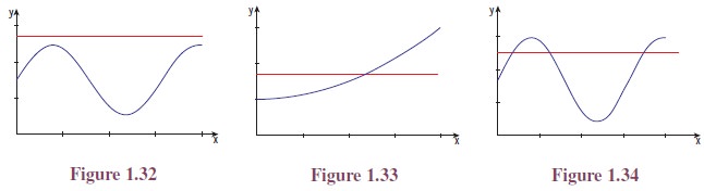
The curve given in Figure 1.32 represents a function from [0, 4] which is not onto if the co-domain contains [1, 3]. The curve given in Figure 1.33 represents a one-to-one function from [0, 4] to R and the curve given in Figure 1.34 represents a function from [0, 4] to R which is not one-to-one.

Testing whether a given curve represents a one-to-one function, onto function or not by drawing horizontal lines is called horizontal line test or simply horizontal test.

Further by seeing the diagrams in Illustration 1.2 and Figures 1.5 to Figure 1.7, the function

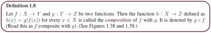
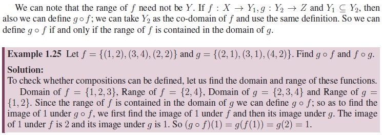
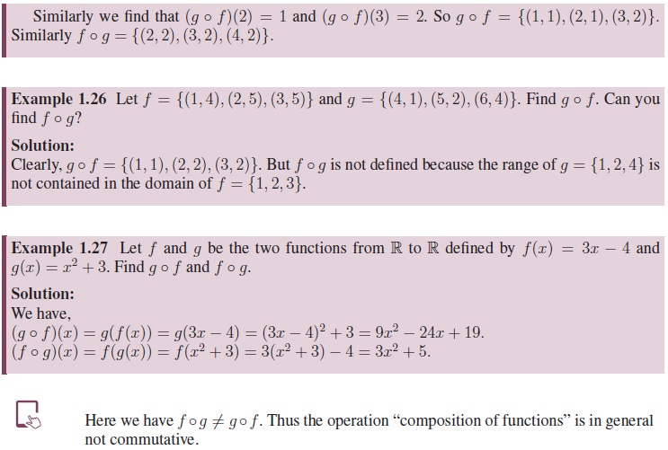
4. Operations on Functions Composition

Let there be two functions f and g as given in the Figure 1.36 and Figure 1.37. Let us note that the co-domain of f and the domain of g are the same. Let us cut off Figure 1.37 of g and paste it on the Figure 1.36 of f so that the domain Y of g is pasted on co-domain Y of f. (See Figure 1.38.)

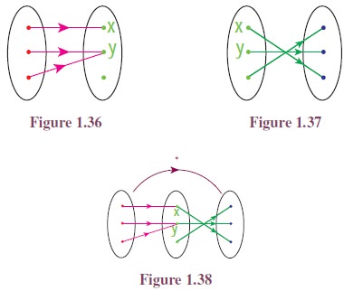
Now we can define a function h : X → Z in a natural way. To find the image of a under h, we first see the image of a under f; it is x; then we see the image of this x under g; this is r. That is, h(a) = r. Similarly, we declare h(b) = q and h(c) = q. In this way we can define a new function h. This h is called the composition of f with g.

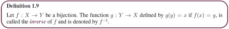
5. Inverse of a Function

Let there be a bijection f : X → Y as given in the Figure 1.41.

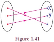
If we look this function in a mirror, we get a function from Y to X. Let us call that function as g.

Then g is a function from Y to X defined by g(x) = b, g(y) = c, g(z) = a.

This function g is an example for the inverse of f. Now we define the inverse of a function.

If a function f has an inverse, then we say that f is invertible. There is a nice relationship between composition of functions and inverse.

Let f : X → Y be a bijection and g : Y → X be its inverse. Then g◦f = IX and f ◦g = IY where IX and IY are identity functions on X and Y respectively. Moreover, if f : X → Y and g : Y → X are functions such that g ◦ f = IX and f ◦ g = IY , then both f and g are bijections and they are inverses to each other; that is f−1 = g and g−1 = f.

Using the discussions above, the terms invertible and inverse can be defined in some other way as follows:

We may use this concept to prove some functions are bijective.

If f is a bijection, then f−1(y) is nothing but the pre-image of y under f. Let us note that the inverses are defined only for bijections. If f is not one-to-one , then there exists a and b such that a ¹ b and f(a) = f(b). Let this value be y. Then we cannot define f−1(y) because both a and b are pre-images of y under f, as f−1 cannot assume two different values for y. If f is not onto, then there will be a y in Y without a pre-image. In this case also we cannot assign any value to f−1(y).

For example, if A = {1, 2, 3, 4} and f = {(1, 2), (2, 4), (3, 1), (4, 3)}. Then the range of f is {1, 2, 3, 4}; the inverse of f is {(1, 3), (2, 1), (3, 4), (4, 2)}.

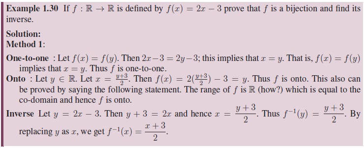
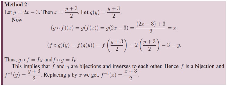
Working Rule to Find the Inverse of Functions from R to R:

Let f : R → R be the given function.

i. write y = f(x);

ii. write x in terms of y;

iii. write f −1(y) = the expression in y.

iv. replace y as x.

6. Algebra of Functions

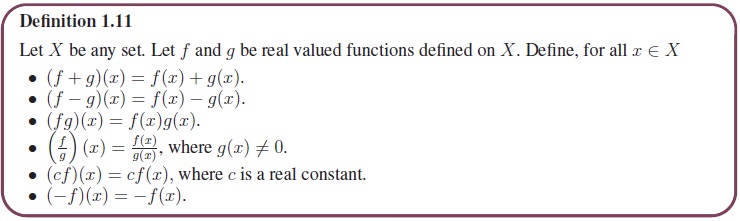
A function whose co-domain is R or a subset of R is called a real valued function. We can discuss many more operations on functions if it is real valued.

Let f and g be two real valued functions. Can we define addition of f and g? Naturally we expect the sum of two functions to be a function. The value of f + g at a point x should be related to the values of f and g at x. So to define f + g at a point x, we must know both f(x) and g(x). In other words x must be in the domain of f as well as in the domain of g. And the natural way of defining + g at x is f(x) + g(x). So if we impose a condition that the domains of f and g to be the same, then we can define f + g. In the same way we can define subtraction, multiplication and many more algebraic operations available on the set R of the real numbers.

Note that the domain may be any set, not necessarily a set of numbers. For example if X is a set of students of a class, f and g functions representing the marks obtained by the students in two tests, then the function f + g represent the total marks of the students in the two tests. It is easy to see that the operations addition, subtraction, multiplication and division defined above satisfy the following properties.

• (f + g) + h = f + (g + h)

• f + g = g + f

• 0 + f = f + 0, where 0 is the zero function defined by 0(x)=0 for all x.

• f + (−f)=(−f) + f = 0

• f(g + h) = fg + fh

• (c1 + c2)f = c1f + c2f where c1 and c2 are real constants.

We can list many more properties of these operations. The proofs are simple; however let us prove only one to show a way in which these properties can be proved.

Let us prove f(g + h) = f g + f h. To prove f(g + h) = f g + f h we have to prove that (f(g + h))(x) = (f g + f h)(x) for all x in the domain.

Theorem 1.3: If f and g are real-valued functions, then f(g + h) = fg + fh.

Proof. Let X be any set and f and g be real-valued functions defined on X. Let x ∈ X.

(f(g + h))(x)

= f(x)(g + h)(x) (by the definition of product)

= f(x)[g(x) + h(x)] (by the definition of addition)

= f(x)g(x) + f(x)h(x) (by the distributivity of reals)

= (fg)(x)+(fh)(x) (by the definition of product)

= (fg + fh)(x) (by the definition of addition)

Thus (f(g + h))(x)=(fg + fh)(x) for all x ∈ X; hence f(g + h) = fg + fh.

7. Some Special Functions

Now let us see some special functions.

(i) The function f : R → R defined by

f(x) = a0xn + a1xn−1 + a2xn−2 + ... + an−1x + an,

where ai are constants, is called a polynomial function. Since the right hand side of the equality defining the function is a polynomial, this function is called a polynomial function.

(ii) The function f : R → R defined by f(x) = ax + b where a = 0 and b are constants, is called a linear function. A function which is not linear is called a non-linear function.

Clearly a linear function is a polynomial function. The graph of this function is a straight line; a straight line is called a linear curve; so this function is called a linear function. (one may come across different definitions for linear functions in higher study of mathematics.)

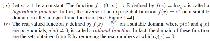
(iii) Let a be a non-negative constant. Consider the function f : R → R defined by f(x) = ax. If a = 0, x ¹ 0 then the function becomes the zero function and if a = 1, then function f : R → R defined by f(x) = ax is the constant function f(x) = 1. [See, Figures 1.42 and 1.43].

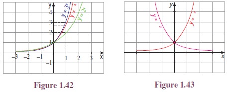
When a > 1, the function f(x) = ax is called an exponential function. Moreover, any function having x in the “power” is called as an exponential function.

The function defined by f(x) = x, f(x) = 2x and f(x) = x3 + 2x are some examples for odd functions. The functions defined by f(x) = x2, f(x) = 3, f(x) = x4 + x2 and f(x) = |x| are some examples for even functions. Note that the function f(x) = x + x2 is neither even nor odd.

We can prove the following results.

i.            The sum of two odd functions is an odd function.

ii.            The sum of two even functions is an even function

iii.            The product of two odd functions is an even function.

iv.            The product of two even functions is an even function.

v.            The product of an odd function and an even function is an odd function.

vi.            The only function which is both odd and even function is the zero function.

vii.            The product of a positive constant and an even function is an even function.

viii.            The product of a negative constant and an even function is also an even function.

ix.            The product of a constant and an odd function is an odd function.

x.            There are functions which are neither odd nor even.

Let us prove one of the above properties. The other properties can be proved similarly.

Theorem 1.4:  The product of an odd function and an even function is an odd function.

Proof. Let f be an odd function and g be an even function. Let h = f g. Now

h(−x) = (f g)(−x) = f(−x)g(−x) = −f(x)g(x) (as f is odd and g is even) = −h(x)

Thus h is an odd function. This shows that f g is an odd function.