Frequency Distribution

Frequency Distribution

A tabular arrangement of raw data by a certain number of classes and the number of items (called frequency) belonging to each class is termed as a frequency distribution. The frequency distributions are of two types, namely, discrete frequency distribution and continuous frequency distribution.

Discrete Frequency Distribution

Raw data sometimes may contain a limited number of values and each of them appeared many numbers of times. Such data may be organized in a tabular form termed as a simple frequency distribution. Thus the tabular arrangement of the data values along with the frequencies is a simple frequency distribution. A simple frequency distribution is formed using a tool called ‘tally chart’. A tally chart is constructed using the following method:

·           Examine each data value.

·           Record the occurrence of the value with the slash symbol (/), called tally bar or tally mark.

·           If the tally marks are more than four, put a crossbar on the four tally bar and make this as block of 5 tally bars (////)

·           Find the frequency of the data value as the total number of tally bars i.e., tally marks corresponding to that value.

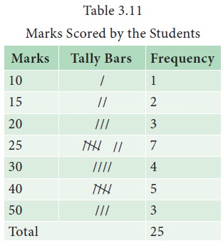
Example 3.11

The marks obtained by 25 students in a test are given as follows: 10, 20, 20, 30, 40, 25, 25, 30, 40, 20, 25, 25, 50, 15, 25, 30, 40, 50, 40, 50, 30, 25, 25, 15 and 40. The following discrete frequency distribution represents the given data:

Continuous Frequency Distribution:

It is necessary to summarize and present large masses of data so that important facts from the data could be extracted for effective decisions. A large mass of data that is summarized in such a way that the data values are distributed into groups, or classes, or categories along with the frequencies is known as a continuous or grouped frequency distribution.

Example 3.12

Table 3.12 displays the number of orders for supply of machineries received by an industrial plant each week over a period of one year.

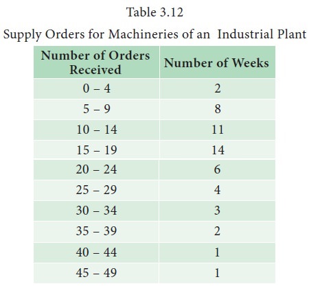
This table is a grouped frequency distribution in which the number of orders are given as classes and number of weeks as frequencies. Some terminologies related to a frequency distribution are given below.

Class: If the observations of a data set are divided into groups and the groups are bounded by limits, then each group is called a class.

Class limits: The end values of a class are called class limits. The smaller value of the class limits is called lower limit (L) and the larger value is called the upper limit(U).

Class interval: The difference between the upper limit and the lower limit is called class interval (I). That is, I = U – L.

Class boundaries: Class boundaries are the midpoints between the upper limit of a class and the lower limit of its succeeding class in the sequence. Therefore, each class has an upper and lower boundaries.

Width : Width of a particular class is the difference between the upper class boundary and lower class boundary.

Mid- point: Half of the difference between the upper class boundary and lower class boundary.

In Example 3.12, the interval 0 - 4 is a class interval with 0 as the lower limit nd 4 as the upper limit. The upper boundary of this class is obtained as midpoint of the upper limit of this class and lower limit of its succeeding class. Thus the upper boundary of the class 0 - 4 is 4.5. The lower class boundary of this is 0 - 0.5 which is - 0.5. The lower boundary of the class 5 - 9 is clearly 4.5. Similarly, the other boundaries of different classes can be found. The width of the classes is 5.

Inclusive and Exclusive Methods of Forming Frequency Distribution

Formation of frequency distribution is usually done by two different methods, namely inclusive method and exclusive method.

Inclusive method

In this method, both the lower and upper class limits are included in the classes. Inclusive type of classification may be used for a grouped frequency distribution for discrete variable like members in a family, number of workers etc., It cannot be used in the case of continuous variable like height, weight etc., where integral as well as fractional values are permissible. Since both upper limit and lower limit of classes are included for frequency calculation, this method is called inclusive method.

Exclusive method

In this method, the values which are equal to upper limit of a class are not included in that class and instead they would be included in the next class. The upper limit is not at all taken into consideration or in other words it is always excluded from the consideration. Hence this method is called exclusive method .

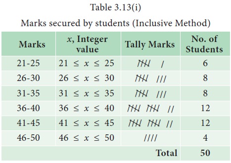
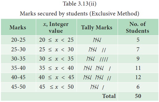
Example 3.13

The marks scored by 50 students in an examination are given as follows:

23, 25, 36, 39, 37, 41, 42, 22, 26, 35, 34, 30, 29, 27, 47, 40, 31, 32, 43, 45, 34, 46, 23, 24, 27, 36, 41, 43, 39, 38, 28, 32, 42, 33, 46, 23, 34, 41, 40, 30, 45, 42, 39, 37, 38, 42, 44, 46, 29, 37.

It can be observed from this data set that the marks of 50 students vary from 22 to 47. If it is decided to divide this group into 6 smaller groups, we can have the boundary lines fixed as 25, 30, 35, 40, 45 and 50 marks. Then, we form the six groups with the boundaries as 21 - 25, 26 - 30, 31 - 35, 36 - 40, 41 – 45 and 46 - 50.

The continuous frequency distribution formed by inclusive and exclusive methods are displayed in Table 3.13(i) and Table 3.13(ii), respectively.

True class intervals

In the case of continuous variables, we take the classes in such a way that there is no gap between successive classes. The classes are defined in such a way that the upper limit of each class is equal to lower limit of the succeeding class. Such classes are known as true classes. The inclusive method of forming class intervals are also known as not-true classes. We can convert the not-true classes into true-classes by subtracting 0.5 from the lower limit of the class and adding 0.5 to the upper limit of each class like 19.5 - 25.5, 25.5 - 30.5, 30.5 – 35.5, 35.5 – 40.5, 40.5 - 45.5, 45.5 – 50.5.

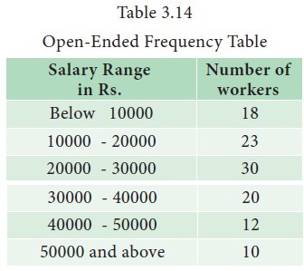
Open End Classes

When a class limit is missing either at the lower end of the first class interval or at the upper end of the last classes or when the limits are not specified at both the ends, the frequency distribution is said to be the frequency distribution with open end classes.

Example 3.14

Salary received by 113 workers in a factory are classified into 6 classes. The classes and their frequencies are displayed in Table 3.14 Since the lower limit of the first class and the upper limit of the last class are not specified, they are open end classes.

Guidelines on Compilation of Continuous Frequency Distribution

The following guidelines may be followed for compiling the continuous frequency distribution.

·           The values given in the data set must be contained within one (and only one) class and overlapping classes must not occur.

·           The classes must be arranged in the order of their magnitude.

·           Normally a frequency distribution may have 8 to 10 classes. It is not desirable to have less than 5 and more than 15 classes.

·           Frequency distributions having equal class widths throughout are preferable. When this is not possible, classes with smaller or larger widths can be used. Open ended classes are acceptable but only in the first and the last classes of the distribution.

·           It should be noted that in a frequency distribution, the first class should contain the lowest value and the last class should contain the highest value.

·           The number of classes may be determined by using the Sturges formula k = 1 + 3.322log10N, where N is the total frequency and k is the number of classes.