Entropy

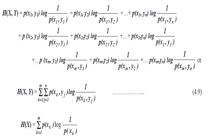
ENTROPY:

The different conditional entropies, Joint and Conditional Entropies:

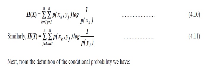
It is clear that all the probabilities encountered in a two dimensional communication system could be derived from the JPM. While we can compare the JPM, therefore, to the impedance or admittance matrices of an n-port electric network in giving a unique description of the system under consideration, notice that the JPM in general, need not necessarily be a square matrix and even if it is so, it need not be symmetric. We define the following entropies, which can be directly computed from the JPM.

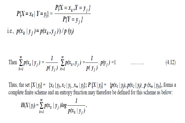
Taking the average of the above entropy function for all admissible characters received, we have the average ― conditional Entropy” or “Equivocation”:

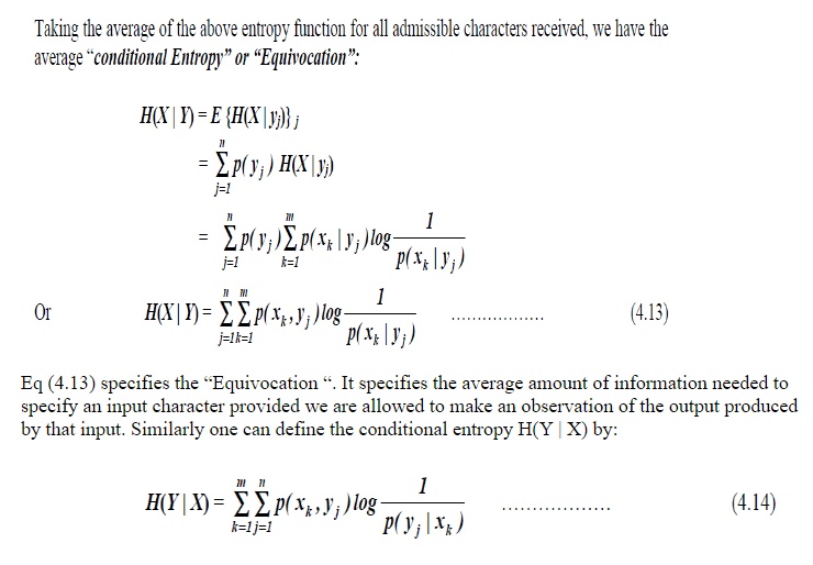
Observe that the manipulations, ' The entropy you want is simply the double summation of joint probability multiplied by logarithm of the reciprocal of the probability of interest‟ . For  example, if you want joint entropy, then the probability of interest will be joint probability. If  you want source entropy, probability of interest will be the source probability. If you want the equivocation or conditional entropy, H (X|Y) then probability of interest will be the conditional probability p (xK |yj) and so on.

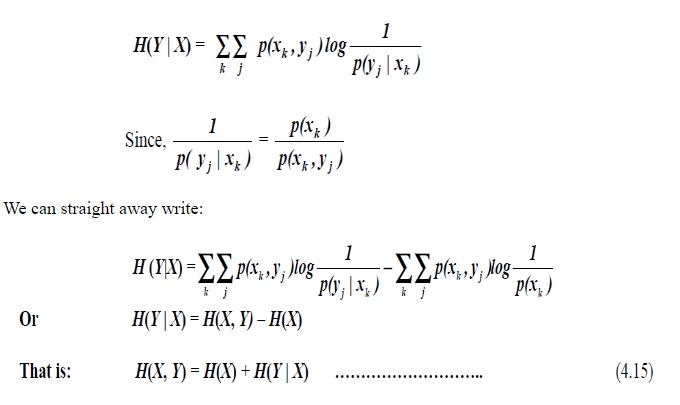
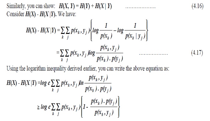
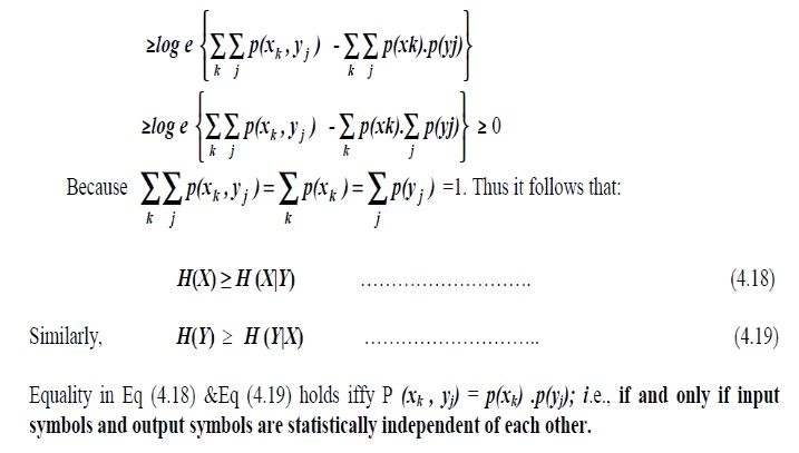
All the five entropies so defined are all inter-related. For example, We have

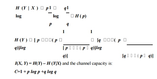
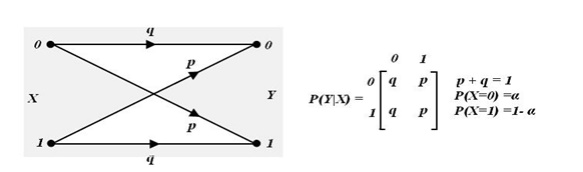
Binary Symmetric Channels (BSC):

The channel is called a 'Binary Symmetric Channel‘ or ( BSC). It is one of the most common and widely used channels. The channel diagram of a BSC is shown in Fig 3.4. Here 'p‘ is called the error probability.

For this channel we have:

In this case it is interesting to note that the equivocation, H (X|Y) =H (Y|X).

An interesting interpretation of the equivocation may be given if consider an idealized communication system with the above symmetric channel.

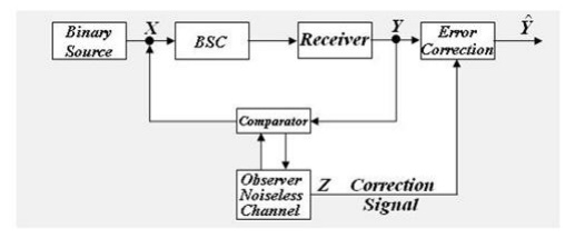
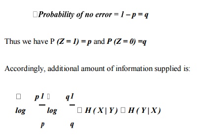
The observer is a noiseless channel that compares the transmitted and the received symbols. Whenever there is an error a ‗ 1‘ is sent to the receiver as a correction signal and  appropriate correction is effected. When there is no error the observer transmits a '0‘ indicating  no change. Thus the observer supplies additional information to the receiver, thus compensating for the noise in the channel. Let us compute this additional information .With P (X=0) = P (X=1) = 0.5, we have:

Probability of sending a „1‟ = Probability of error in the channel .

Probability of error = P (Y=1|X=0).P(X=0) + P

(Y=0|X=1).P(X=1) = p × 0.5 +

p × 0.5 = p

Thus the additional information supplied by the observer is exactly equal to the equivocation of the source. Observe that if ‗ p‘ and ‗ q‘ are interchanged in the channel matrix, the trans - information of the channel remains unaltered. The variation of the mutual information with the  probability of error is shown in Fig 3.6(a) for P (X=0) = P (X=1) = 0.5. In Fig 4.6(b) is shown the dependence of the mutual information on the source probabilities.

Binary Erasure Channels (BEC):

BEC is one of the important types of channels used in digital communications. Observe that whenever    an      error occurs,y‘ theand symbolnodecisionwill be about the information but an immediate request will be made for retransmission, rejecting what       have been received (ARQ techniques), thus ensuring 100% correct data recovery. Notice that this   channel also is a symmetric channel and we have with P(X = 0) =

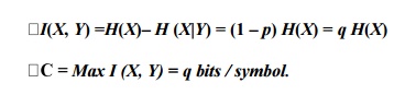
In this particular case, use of the equation I(X, Y) = H(Y) – H(Y | X) will not be correct, as H(Y) involves "y‘ and the information given by " y‘ is rejected at the receiver.