Echelon form and finding the rank of the matrix (upto the order of 3×4)

Echelon form and finding the rank of the matrix (upto the order of 3×4)

A matrix A of order m × n is said to be in echelon form if

(i) Every row of A which has all its entries 0 occurs below every row which has a non-zero entry.

(ii) The number of zeros before the first non-zero element in a row is less then the number of such zeros in the next row.

Example 1.6

Find the rank of the matrix A=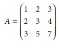 

Solution :

The order of A is 3 × 3.

∴ ρ(A) ≤ 3.

Let us transform the matrix A to an echelon form by using elementary transformations.

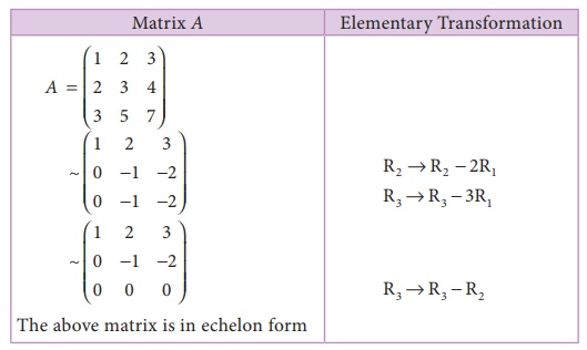
The number of non zero rows is 2

∴Rank of A is 2.

ρ (A) = 2.

Note

A row having atleast one non -zero element is called as non-zero row.

Example 1.7

Find the rank of the matrix A=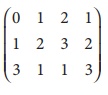 

Solution:

The order of A is 3 × 4.

∴ ρ (A)≤3.

Let us transform the matrix A to an echelon form

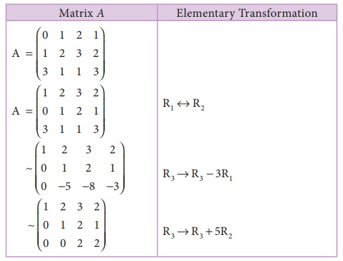
The number of non zero rows is 3. ∴ ρ(A) =3.

Example 1.8

Find the rank of the matrix A=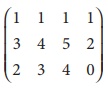 

Solution:

The order of A is 3 × 4.

∴ ρ(A) ≤ 3.

Let us transform the matrix A to an echelon form

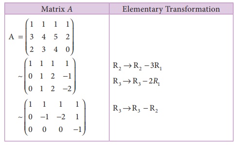
The number of non zero rows is 3.

∴ ρ (A) =3.

Consistency of Equations

System of linear equations in two variables

We have already studied , how to solve two simultaneous linear equations by matrix inversion method.

Recall

Linear equations can be written in matrix form AX=B, then the solution is X = A⁻¹B , provided |A| ≠0

Consider a system of linear equations with two variables,

 ax + by + h

 cx + dy + k (1)

Where a, b, c, d, h and k are real constants and neither a and b nor c and d are both zero.

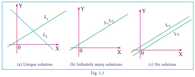
For any tow given lines L₁ and L₂, one and only one of the following may occur.

L₁ and L₂ intersect at exactly one point

L₁ and L₂ are coincident

L₁ and L₂ are parallel and distinct.

(see Fig 1.1) In the first case, the system has a unique solution corresponding to the single point of intersection of the two lines.

In the second case, the system has infinitely many solutions corresponding to the points lying on the same line

Finally in the third case, the system has no solution because the two lines do not intersect.

Let us illustrate each of these possibilities by considering some specific examples.

(a) A system of equations with exactly one solution

Consider the system 2x − y = 1, 3x + 2 y = 12 which represents two lines intersecting at (2, 3) i.e (2, 3) lies on both lines. So the equations are consistent and have unique solution.

(b) A system of equations with infinitely many solutions

Consider the system 2x − y = 1, 6x − 3y = 3 which represents two coincident lines. We find that any point on the line is a solution. The equations are consistent and have infinite sets of solutions such as (0, −1), (1, 1) and so on. Such a system is said to be dependent.

(c) A system of equations that has no solution

Consider the system 2x − y = 1, 6x − 3y = 12 which represents two parallel straight lines. The equations are inconsistent and have no solution.

System of non Homogeneous Equations in three variables

A linear system composed of three linear equations with three variables x, y and z has the general form

a₁ x + b₁ y + c₁ z = d₁

a₂ x + b₂y + c₂z = d₂ (2)

a₃ x + b₃ y + c₃ z = d₃

A linear equation ax + by + cz = d (a, b and c not all equal to zero) in three variables represents a plane in three dimensional space. Thus, each equation in system (2) represents a plane in three dimensional space, and the solution(s) of the system is precisely the point(s) of intersection of the three planes defined by the three linear equations that make up the system. This system has one and only one solution, infinitely many solutions, or no solution, depending on whether and how the planes intersect one another. Figure 1.2 illustrates each of these possibilities.

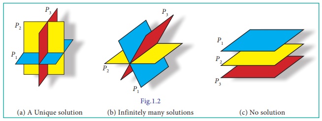
In Figure 1.2(a), the three planes intersect at a point corresponding to the situation in which system (2) has a unique solution.

Figure 1.2 (b) depicts a situation in which there are infinitely many solutions to the system. Here the three planes intersect along a line, and the solutions are represented by the infinitely many points lying on this line.

In Figure 1.2 (c), the three planes are parallel and distinct, so there is no point in common to all three planes; system (2) has no solution in this case.

Note

Every system of linear equations has no solution, or has exactly one solution or has  infinitely many solutions.

An arbitrary system of ‘m’ linear equations in ‘n’ unknowns can be written as

a₁₁ x₁ + a ₁₂ x₂ + ... + a_1n x_n =b₁

a₂₁ x₁ + a ₂₂ x₂ + ... + a_2n x_n =b₂

.          .              …      .          .

.          .              …      .          .

.          .              …      .          .

a_m1 x₁ + a_{m 2} x₂ + ... + a_mn x_n = b_m

where x₁, x₂,.., x_n are the unknowns and the subscripted a’s and b’s denote the constants.

Augmented matrices

A system of ‘m’ linear equations in ‘n’ unknowns can be abbreviated by writing only the rectangular array of numbers.

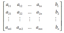
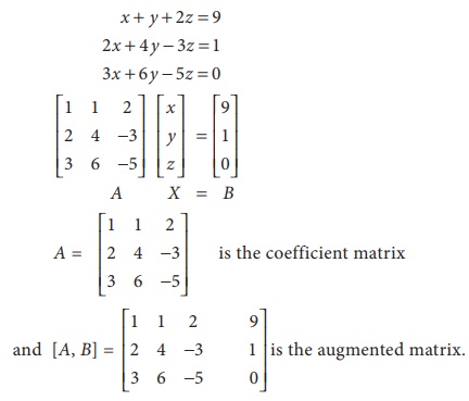
This is called the augmented matrix for the system and 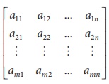 is the coefficient matrix.

Consider the following system of equations