Breadth First Traversal

BREADTH FIRST TRAVERSAL:

Breadth-first search starts at a given vertex s, which is at level 0. In the first stage, we visit all the vertices that are at the distance of one edge away. When we visit there, we paint as "visited," the vertices adjacent to the start vertex s - these vertices are placed into level 1. In the second stage, we visit all the new vertices we can reach at the distance of two edges away from the source vertex s. These new vertices, which are adjacent to level 1 vertices and not previously assigned to a level, are placed into level 2, and so on. The BFS traversal terminates when every vertex has been visited.

To keep track of progress, breadth-first-search colors each vertex. Each vertex of the graph is in one of three states:

1.     Undiscovered;

2.     Discovered but not fully explored; and

3.  Fully explored.

The state of a vertex, u, is stored in a color variable as follows:

1.     color[u] = White - for the "undiscovered" state,

2.     color [u] = Gray - for the "discovered but not fully explored" state, and

3.     color [u] = Black - for the "fully explored" state.

The BFS(G, s) algorithm develops a breadth-first search tree with the source vertex, s, as its root. The parent or predecessor of any other vertex in the tree is the vertex from which it was first discovered. For each vertex, v, the parent of v is placed in the variable π[v]. Another variable, d[v], computed by BFS contains the number of tree edges on the path from s to v. The breadth-first search uses a FIFO queue, Q, to store gray vertices.

Algorithm: Breadth-First Search Traversal

BFS(V, E, s)

1.      for each u in V − {s}     ▷ for each vertex u in V[G] except s.

2.                         do color[u] ← WHITE

3.       d[u] ← infinity    

4.       π[u] ← NIL

5.       color[s] ← GRAY          ▷ Source vertex discovered

6.       d[s] ← 0     ▷ initialize

7.       π[s] ← NIL ▷ initialize

8.       Q ← {}       ▷ Clear queue Q

9.       ENQUEUE(Q, s)

10      while Q is non-empty   

11.     do u ← DEQUEUE(Q) 

12.     for each v adjacent to u 

13.     do if color[v] ← WHITE        

14.     then color[v] ← GRAY

15.     d[v] ← d[u] + 1   

16.     π[v] ← u    

17.     ENQUEUE(Q, v)

18.     DEQUEUE(Q)    

19.     color[u] ← BLACK

Example:

The following figure illustrates the progress of breadth-first search on the undirected sample graph.

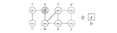
a. After initialization (paint every vertex white, set d[u] to infinity for each vertex u, and set the parent of every vertex to be NIL), the source vertex is discovered in line 5. Lines 8-9 initialize Q to contain just the source vertex s.

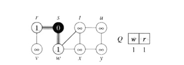
b. The algorithm discovers all vertices 1 edge from s i.e., discovered all vertices (w and r) at level 1.

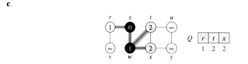
d. The algorithm discovers all vertices 2 edges from s i.e., discovered all vertices (t, x, and v) at level 2.

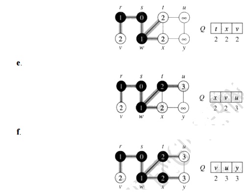
g. The algorithm discovers all vertices 3 edges from s i.e., discovered all vertices (u and y) at level 3.

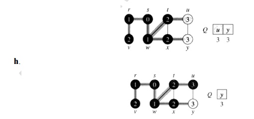
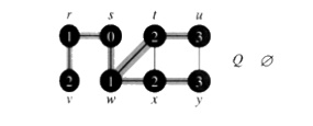
i. The algorithm terminates when every vertex has been fully explored.