Additional White Box Test Design Approaches

Additional White Box Test Design Approaches

In addition to methods that make use of software logic and control structures to guide test data generation and to evaluate test completeness there are alternative methods that focus on other characteristics of the code. One widely used approach is centered on the role of variables (data) in the code. Another is fault based. The latter focuses on making modifications to the software, testing the modified version, and comparing results. These will be described in the following sections of this chapter.

Data Flow and White Box Test Design

In order to discuss test data generation based on data flow information, some basic concepts that define the role of variables in a software component need to be introduced.

We say a variable is defined in a statement when its value is assigned or changed.

For example in the statements

the variable Y is defined, that is, it is assigned a new value. In data flow notation this is indicated as a def for the variable Y.

We say a variable is used in a statement when its value is utilized in a statement. The value of the variable is not changed.

A more detailed description of variable usage is given by Rapps and Weyuker [4]. They describe a predicate use (p-use) for a variable that indicates its role in a predicate. A computational use (c-use) indicates the variable‘s role as a part of a computation. In both cases the variable value is unchanged. For example, in the statement

Y =26*X

the variable X is used. Specifically it has a c-use. In the statement if (X >98)

Y= max

X has a predicate or p-use. There are other data flow roles for variables such as undefined or dead, but these are not relevant to the subsequent discussion. An analysis of data flow patterns for specific variables is often very useful for defect detection. For example, use of a variable without a definition occurring first indicates a defect in the code. The variable has not been initialized. Smart compilers will identify these types of defects. Testers and developers can utilize data flow tools that will identify and display variable role information. These should also be used prior to code reviews to facilitate the work of the reviewers.

Using their data flow descriptions, Rapps and Weyuker identified several data-flow based test adequacy criteria that map to corresponding coverage goals. These are based on test sets that exercise specific path segments, for example:

All def

All p-uses

All c-uses/some p-uses

All p-uses/some c-uses

All uses

All def-use paths

The strongest of these criteria is all def-use paths. This includes all p- and c-uses.

We say a path from a variable definition to a use is called a def-use path.

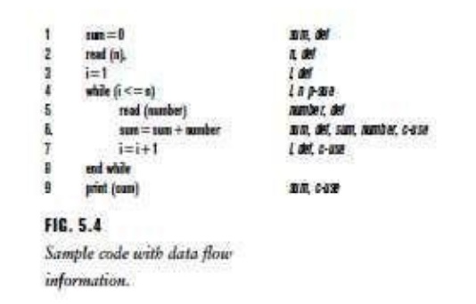
To satisfy the all def-use criterion the tester must identify and classify occurrences of all the variables in the software under test. A tabular summary is useful. Then for each variable, test data is generated so that all definitions and all uses for all of the variables are exercised during test. As an example we will work with the code in Figure 5.4 that calculates the sum of n numbers.

The variables of interest are sum, i, n, and number. Since the goal is to satisfy the all def-use criteria we will need to tabulate the def-use occurrences for each of these variables. The data flow role for each variable in each statement of the example is shown beside the statement in italics.

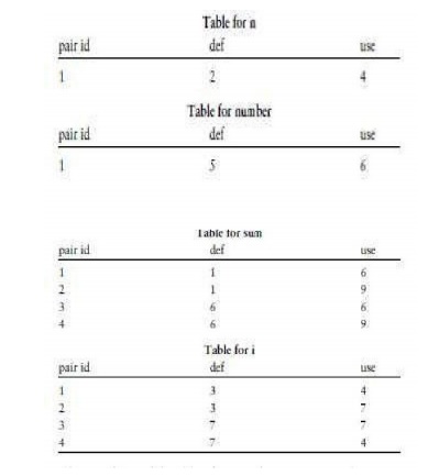
Tabulating the results for each variable we generate the following tables. On the table each defuse pair is assigned an identifier. Line numbers are used to show occurrence of the def or use. Note that in some statements a given variable is both defined and used.

After completion of the tables, the tester then generates test data to exercise all of these def-use pairs In many cases a small set of test inputs will cover several or all def-use paths. For this example two sets of test data would cover all the def-use pairs for the variables:

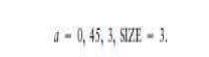
Test data set 1: n 0

Test data set 2: n 5, number 1,2,3,4,5

Set 1 covers pair 1 for n, pair 2 for sum, and pair 1 for i. Set 2 covers pair 1 for n, pair 1 for number, pairs 1,3,4 for sum, and pairs 1,2,3,4 for i.

Note even for this small piece of code there are four tables and four def-use pairs for two of the variables.

As with most white box testing methods, the data flow approach is most effective at the unit level of testing. When code becomes more complex and there are more variables to consider it becomes more time consuming for the tester to analyze data flow roles, identify paths, and design the tests. Other problems with data flow oriented testing occur in the handling of dynamically bound variables such as pointers. Finally, there are no commercially available tools that provide strong support for data flow testing, such as those that support control-flow based testing. In the latter case, tools that determine the degree of coverage, and which portions of the code are yet uncovered, are of particular importance. These are not available for data flow methods. For examples of prototype tools.

Loop Testing

Loops are among the most frequently used control structures. Experienced software engineers realize that many defects are associated with loop constructs. These are often due to poor programming practices and lack of reviews. Therefore, special attention should be paid to loops during testing. Beizer has classified loops into four categories: simple, nested, concatenated, and unstructured [4]. He advises that if instances of unstructured loops are found in legacy code they should be redesigned to reflect structured programming techniques. Testers can then focus on the remaining categories of loops.

Loop testing strategies focus on detecting common defects associated with these structures. For example, in a simple loop that can have a range of zero to n iterations, test cases should be developed so that there are:

(i) zero iterations of the loop, i.e., the loop is skipped in its entirely;

(ii) one iteration of the loop;

(iii) two iterations of the loop;

(iv)k iterations of the loop where k n;

(v)             n 1 iterations of the loop;

(vi)n 1 iterations of the loop (if possible).

If the loop has a nonzero minimum number of iterations, try one less than the minimum. Other cases to consider for loops are negative values for the loop control variable, and n 1 iterations of the loop if that is possible. Zhu has described a historical loop count adequacy criterion that states that in the case of a loop having a maximum of n iterations, tests that execute the loop zero times, once, twice, and so on up to n times are required.

Beizer has some suggestions for testing nested loops where the outer loop control variables are set to minimum values and the innermost loop is exercised as above. The tester then moves up one loop level and finally tests all the loops simultaneously. This will limit the number of tests to perform; however, the number of test under these circumstances is still large and the tester may have to make trade-offs. Beizer also has suggestions for testing concatenated loops.

Mutation Testing

Mutation testing is another approach to test data generation that requires knowledge of code structure, but it is classified as a fault-based testing approach. It considers the possible faults that could occur in a software component as the basis for test data generation and evaluation of testing effectiveness.

Mutation testing makes two major assumptions:

1.  The competent programmer hypothesis. This states that a competent programmer writes programs that are nearly correct. Therefore we can assume that there are no major construction errors in the program; the code is correct except for a simple error(s).

2.  The coupling effect. This effect relates to questions a tester might have about how well mutation testing can detect complex errors since the changes made to the code are very simple. DeMillo has commented on that issue as far back as 1978 [10]. He states that test data that can distinguish all programs differing from a correct one only by simple errors are sensitive enough to distinguish it from programs with more complex errors.

Mutation testing starts with a code component, its associated test cases, and the test results.

The original code component is modified in a simple way to provide a set of similar components that are called mutants. Each mutant contains a fault as a result of the modification. The original test data is then run with the mutants. If the test data reveals the fault in the mutant (the result of the modification) by producing a different output as a result of execution, then the mutant is said to be killed. If the mutants do not produce outputs that differ from the original with the test data, then the test data are not capable of revealing such defects. The tests cannot distinguish the original from the mutant. The tester then must develop additional test data to reveal the fault and kill the mutants. A test data adequacy criterion that is applicable here is the following:

A test set T is said to be mutation adequate for program P provided that for every in equivalent mutant Pi of P there is an element t in T such that Pi(t) is not equal to P(t).

The term T represents the test set, and t is a test case in the test set. For the test data to be adequate according to this criterion, a correct program must behave correctly and all incorrect programs behave incorrectly for the given test data.

Mutations are simple changes in the original code component, for example: constant replacement, arithmetic operator replacement, data statement alteration, statement deletion, and logical operator replace- ment. There are existing tools that will easily generate mutants. Tool users need only to select a change operator. To illustrate the types of changes made in mutation testing we can make use of the code in Figure 5.2. A first mutation could be to change line 7 from

If we rerun the tests used for branch coverage as in Table 5.1 this mutant will be killed, that is, the output will be different than for the original code. Another change we could make is in line 5, from

This mutant would also be killed by the original test data. Therefore, we can assume that our original tests would have caught this type of defect. However, if we made a change in line 5 to read

this mutant would not be killed by our original test data in Table 5.1. Our inclination would be to augment the test data with a case that included a zero in the array elements, for example:

However, this test would not cause the mutant to be killed because adding a zero to the output variable sum does not change its final value. In this case it is not possible to kill the mutant. When this occurs, the mutant is said to be equivalent to the original program. To measure the mutation adequacy of a test set T for a program P we can use what is called a mutation score (MS), which is calculated as

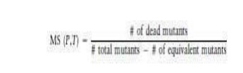
Equivalent mutants are discarded from the mutant set because they do not contribute to the adequacy of the test set. Mutation testing is useful in that it can show that certain faults as represented in the mutants are not likely to be present since they would have been revealed by test data. It also helps the tester to generate hy- potheses about the different types of possible faults in the code and to develop test cases to reveal them. As previously mentioned there are tools to support developers and testers with producing mutants. In fact, many hundreds of mutants can be produced easily. However, running the tests, analyzing results, and developing additional tests, if needed, to kill the mutants are all time consuming. For these reasons mutation testing is usually applied at the unit level. However, recent research in an area called interface mutation (the application of mutation testing to evaluate how well unit interfaces have been tested) has suggested that it can be applied effectively at the integration test level as well

.Mutation testing as described above is called strong mutation testing. There are variations that reduce the number of mutants produced. One of these is called weak mutation testing which focuses on specific code components .