Spice Tutorial

SPICE TUTORIAL

1. Introduction

Given below is a brief introduction to simulation using HSPICE and AWAVES/Cosmoscope in the UTD network.

HSPICE is a device level circuit simulator from Synopsys.

HSPICE takes a SPICE file as input and produces output describing the requested simulation of the circuit.

The simulation output can be viewed with AWAVES (or) Cosmos cope from Synopsys. A short example is provided to illustrate the basic procedures involved in running HSPICE.

2. Setting up your account to access HSPICE

This section shows how to setup your environment for running HSPICE.

For users who have a working CAD setup, you may just want to check that the LM_LICENSE_FILE has the following values in the list of all the other licenses,/home/cad/flexlm/ti-license:/home/cad/flexlm/hspice.flx.

If not, follow the procedures below: Instructions for both bash and tcsh/csh users is provided here:

bash users:

Add the following line to the .bash_profile

LM_LICENSE_FILE=$LM_LICENSE_FILE:/home/cad/flexlm/hspice.flx ; export

LM_LICENSE_FILE

tcsh/csh users:

Add the following line to your

.tcshrc

setenv

LM_LICENSE_FILE ${LM_LICENSE_FILE}:/home/cad/flexlm/hspice.flx

To test if the above procedure has setup your environment successfully, invoke a new shell (this will ensure that the new environment variables are in place).

Also you will need a HSPICE input file to test this (You can copy paste the HSPICE example given below to test this). The input Spice file is typically named with extension *.sp.

% hspice<your_input_file>.sp

The following message indicates trouble with invocation:

If the error is "hspice: command not found" make sure that the HSPICE directory " /home/cad/synopsys/hspice/U-2003.09-SP1/sun58/" is included in the $PATH variable.

Cannot execute /home/cad/synopsys/hspice/U-2003.09-SP1/sun58/hspice

or

lic: Using FLEXlm license file:

lic: /home/cad/flexlm/hspice.flx

lic: Unable to checkout hsptest

The above error may indicate that the license server maybe down, or the machine is not able to run HSPICE.

On the other hand if the procedure was successful, you will simply see a message indicating successful completion of simulation or errors in simulation, both of which indicate HSPICE has run your file.

3. Setting up the HSPICE input file

Consider a self loaded min geometry inverter circuit.

The objective of the HSPICE input file below is to measure the tpLH     and tpHL both

graphically and otherwise.

The following HSPICE file is stored in "inv.sp".

The HSPICE input file is commented adequately about the different options used in it.

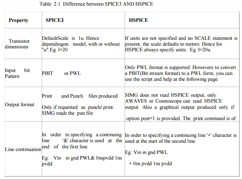
It  will  be  beneficial  to  keep  in  mind  the  following  differences  between  SPICE3  and HSPICE.

HSPICE Example File

*        Self loaded min geometry inverter, sample HSPICE file

*        Include the model files

*        Include the hspice model files for 0.18u technology.

.include  /home/cad/vlsi/models/hspice/cmos0.18um.model

*        The subcircuit for the inverter

.subckt invert in outvddgnd

.param length=0.2u

m01 out in vddvddpfet w='4*length' l='length' m02 out in gndgndnfet w='1.5*length' l='length'

.ends

*        The main inverter

X1 in outvddgnd invert

* Four loads for the inverter

X2 out out1 vddgnd invert X3 out out2 vddgnd invert X4 out out3 vddgnd invert X5 out out4 vddgnd invert

*        PWL pattern for the input, represents a bit stream 1100101

*        Slew=1ns, bit time=5ns

Vin in gnd PWL 0ns pvdd 1ns pvdd 5ns pvdd 6ns pvdd 7ns 0 10ns 0 + 15ns 0 16ns pvdd 21ns pvdd 22ns 0 25ns 0 26ns pvdd *Parametricdefinitions

.parampvdd=2.0v

*        Power supplies vvddvdd 0 pvddvgndgnd 0 0

*        Control statements

.option post=1

.TR 0.05ns 30ns

.print TR V(in out)

*        Measure statements help in calculating TPLH, TPHL etc, without

*        opening the waveform viewer

.measure trantplh trig v(in) val='0.5*pvdd' fall=1 targ v(out) val='0.5*pvdd' rise=1

.measure trantphl trig v(in) val='0.5*pvdd' rise=1 targ v(out) val='0.5*pvdd' fall=1

.END

4. Running HSPICE simulations

The following commands can be used to simulate the above HSPICE file stored in inv.sp and store all the simulation results with file prefix as "inv"

% hspiceinv.sp -o inv

This results in the creation of the following output files: inv.ic -> Operating point node voltages (initial conditions) inv.lis -> Output listing

inv.mt0 -> Transient analysis measurement results

inv.pa0 ->Subcircuit cross-listing

inv.st0 -> Output status

inv.tr0 -> Transient analysis results

5. Analyzing the outputs

In the above example, the output data can be analyzed both graphically as well as in text form.

Text outputs:

To view the results of the .measure computation, execute:

%  cat inv.mt0

$DATA1 SOURCE='HSPICE' VERSION='2003.09-SP1'

.TITLE ' '

tplh   tphl   temper        alter#

3.416e-10  1.002e-09     25.0000      1.0000

As can be seen above, the values of propogation delay have been obtained even before the waveform analysis software has been opened.

Graphical outputs:

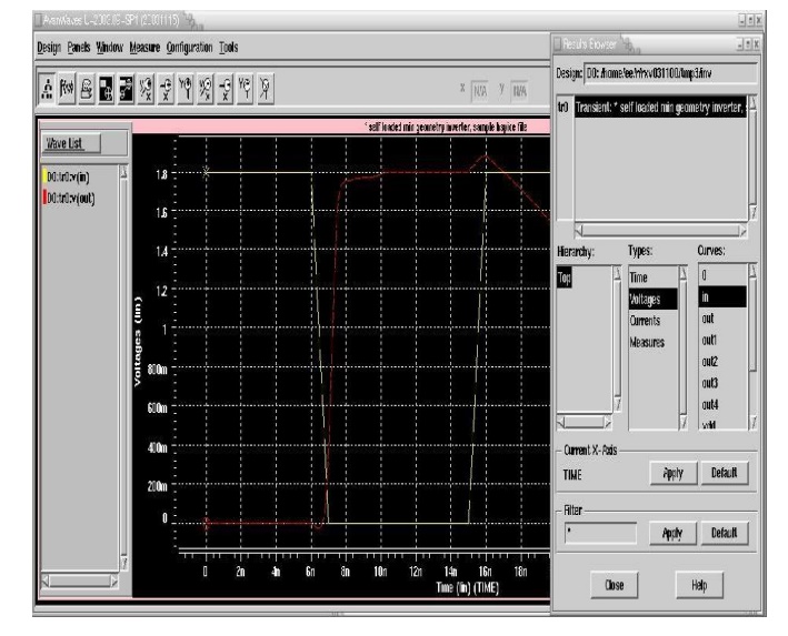
I. Synopsys Awaves:

To invoke AWAVES run the following command:

% awaves

If you get the error "awaves: command not found" make sure that the AWAVES directory "/home/cad/synopsys/hspice/U-2003.09-SP1/sun58/" is included in the $PATH variable.

Once invoked, open the designusing the pull down menu options: Design->Open and select inv.sp and then highlight the tr0 (Transient response)

item in the select box.

You will also see the hierarchy of the netlist and the types of analysis and the individual signals in separate lists in the window. Select Hierarchy -> Top, Types -> Voltages and select the voltages you want to observe.

For eg.in and out by double clicking on the names. You will see the screen below for the stimulus provided in inv.sp.

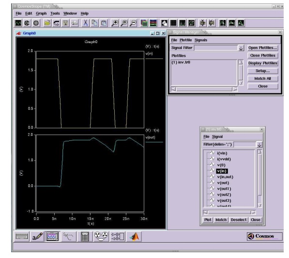
II. Synopsys Cosmoscope:

To invoke Cosmoscope run the following command:

%cscope

If you get the error "awaves: command not found" make sure that the AWAVES directory "

/home/cad/synopsys/cosmo/ai_bin/" is included in the $PATH variable.

Once invoked, open the design using the pull down menu options: File -> Open -> Plot files and select file inv.tr0 in the working directory.

A Signal Manager Window and signal window opens.

Select the necessary signals to be plotted by double-clicking them. For example v(in) and v(out) by double clicking on the signal names in the signal window

You will see the screen below for the stimulus provided in invest.