Software Pipelining Algorithm

Software Pipelining

1 Introduction

2 Software Pipelining of Loops

3 Register Allocation and Code Generation

4 Do-Across Loops

5 Goals and Constraints of Software Pipelining

6 A Software-Pipelining Algorithm

7 Scheduling Acyclic Data-Dependence Graphs

8 Scheduling Cyclic Dependence Graphs

9 Improvements to the Pipelining Algorithms

10Modular Variable Expansion

11 Conditional Statements

12 Hardware Support for Software Pipelining

13 Exercises for Section 10.5

As discussed in the introduction of this chapter, numerical applications tend to have much parallelism. In particular, they often have loops whose iterations are completely independent of one another. These loops, known as do-all loops, are particularly attractive from a parallelization perspective because their iter-ations can be executed in parallel to achieve a speed-up linear in the number of iterations in the loop. Do-all loops with many iterations have enough par-allelism to saturate all the resources on a processor. It is up to the scheduler to take full advantage of the available parallelism. This section describes an al-gorithnij known as software pipelining, that schedules an entire loop at a time, taking full advantage of the parallelism across iterations.

1. Introduction

We shall use the do-all loop in Example 10.12 throughout this section to explain software pipelining. We first show that scheduling across iterations is of great importance,  because there is relatively little parallelism among operations in  a single iteration.  Next, we show that  loop unrolling improves performance by overlapping the computation of unrolled iterations. However, the boundary of the unrolled loop still poses as a barrier to code motion, and unrolling still leaves a lot of performance "on the table." The technique of software pipelining, on the other hand, overlaps a number of consecutive iterations continually until it runs out of iterations. This technique allows software pipelining to produce highly efficient and compact code.

Example 10 . 12 :  Here is a typical do-all loop:

for (i = 0; i < n; i++)

D[i]  = A[i]*B[i]  + c;

Iterations in the above loop write to different memory locations, which are themselves distinct from any of the locations read. Therefore, there are no memory dependences between the iterations, and all iterations can proceed in parallel.

We adopt the following model as our target machine throughout this section. In this model

•             The machine can issue in a single clock: one load, one store, one arithmetic operation, and one branch operation.

•             The machine has a loop-back operation of the form

BL R,  L

which decrements register R and, unless the result is 0, branches to loca-

tion  L.

•              Memory operations have an auto-increment addressing mode, denoted by

++                 after the register.  The register is automatically incremented to point

to the next consecutive address after each access.

•              The arithmetic operations are fully pipelined; they can be initiated every clock but their results are not available until 2 clocks later. All other instructions have a single-clock latency.

If iterations are scheduled one at a time, the best schedule we can get on our machine model is shown in Fig. 10.17. Some assumptions about the layout of the data also also indicated in that figure: registers Rl, R2, and R3 hold the addresses of the beginnings of arrays A, B, and D, register R4 holds the constant c, and register RIO holds the value n — 1, which has been computed outside the loop. The computation is mostly serial, taking a total of 7 clocks; only the loop-back instruction is overlapped with the last operation in the iteration.

//        Rl,  R2,  R3 = &A,  &B,  &D

//        R4     =       c

//        RIO   =       n-1

L:      LD R5, 0(R1++) LD R6, 0(R2++) MUL R7, R5, R6 nop

ADD R8, R7, R4 nop

ST     0(R3++),  R8        BL  RIO,  L

Figure 10.17:  Locally scheduled code for Example 10.12

In general, we get better hardware utilization by unrolling several iterations of a loop. However, doing so also increases the code size, which in turn can have a negative impact on overall performance. Thus, we have to compromise, picking a number of times to unroll a loop that gets most of the performance im-provement, yet doesn't expand the code too much. The next example illustrates the tradeoff.

Example 10.13 : While hardly any parallelism can be found in each iteration of the loop in Example 10.12, there is plenty of parallelism across the iterations.

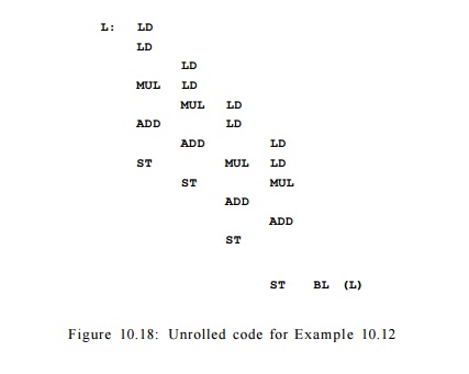
Loop unrolling places several iterations of the loop in one large basic block, and a simple list-scheduling algorithm can be used to schedule the operations to execute in parallel. If we unroll the loop in our example four times and apply Algorithm 10.7 to the code, we can get the schedule shown in Fig. 10.18. (For simplicity, we ignore the details of register allocation for now). The loop executes in 13 clocks, or one iteration every 3.25 clocks.

A loop unrolled k times takes at least 2ft + 5 clocks, achieving a throughput of one iteration every 2 + 5/k clocks. Thus, the more iterations we unroll, the faster the loop runs. As n -» oo, a fully unrolled loop can execute on average an iteration every two clocks. However, the more iterations we unroll, the larger the code gets. We certainly cannot afford to unroll all the iterations in a loop. Unrolling the loop 4 times produces code with 13 instructions, or 163% of the optimum; unrolling the loop 8 times produces code with 21 instructions, or 131% of the optimum. Conversely, if we wish to operate at, say, only 110% of the optimum, we need to unroll the loop 25 times, which would result in code with 55 instructions. •

2. Software Pipelining of Loops

Software pipelining provides a convenient way of getting optimal resource usage and compact code at the same time. Let us illustrate the idea with our running example.

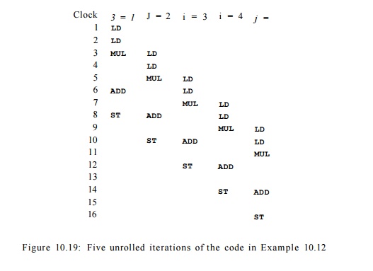
E x a m p l e 1 0 . 1 4 : In Fig. 10.19 is the code from Example 10.12 unrolled five times. (Again we leave out the consideration of register usage.) Shown in row i are all the operations issued at clock i; shown in column j are all the operations from iteration j. Note that every iteration has the same schedule relative to its beginning, and also note that every iteration is initiated two clocks after the preceding one. It is easy to see that this schedule satisfies all the resource and data-dependence constraints.

We observe that the operations executed at clocks 7 and 8 are the same as those executed at clocks 9 and 10. Clocks 7 and 8 execute operations from the first four iterations in the original program. Clocks 9 and 10 also execute operations from four iterations, this time from iterations 2 to 5. In fact, we can keep executing this same pair of multi-operation instructions to get the effect of retiring the oldest iteration and adding a new one, until we run out of iterations.

Such dynamic behavior can be encoded succinctly with the code shown in Fig. 10.20, if we assume that the loop has at least 4 iterations. Each row in the figure corresponds to one machine instruction. Lines 7 and 8 form a 2-clock loop, which is executed n - 3 times, where n is the number of iterations in the original loop.

The technique described above is called software pipelining, because it is the software analog of a technique used for scheduling hardware pipelines. We can think of the schedule executed by each iteration in this example as an 8-stage pipeline. A new iteration can be started on the pipeline every 2 clocks. At the beginning, there is only one iteration in the pipeline. As the first iteration proceeds to stage three, the second iteration starts to execute in the first pipeline stage.

By clock 7, the pipeline is fully filled with the first four iterations. In the steady state, four consecutive iterations are executing at the same time. A new iteration is started as the oldest iteration in the pipeline retires. When we run out of iterations, the pipeline drains, and all the iterations in the pipeline run to completion. The sequence of instructions used to fill the pipeline, lines 1 through 6 in our example, is called the prolog; lines 7 and 8 are the steady state; and the sequence of instructions used to drain the pipeline, lines 9 through 14, is called the epilog.

For this example, we know that the loop cannot be run at a rate faster than 2 clocks per iteration, since the machine can only issue one read every clock, and there are two reads in each iteration. The software-pipelined loop above executes in 2n + 6 clocks, where n is the number of iterations in the original loop. As n oo, the throughput of the loop approaches the rate of one iteration every two clocks. Thus, software scheduling, unlike unrolling, can potentially encode the optimal schedule with a very compact code sequence.

Note that the schedule adopted for each individual iteration is not the shortest possible. Comparison with the locally optimized schedule shown in Fig. 10.17 shows that a delay is introduced before the ADD operation. The delay is placed strategically so that the schedule can be initiated every two clocks without resource conflicts. Had we stuck with the locally compacted schedule, the initiation interval would have to be lengthened to 4 clocks to avoid resource conflicts, and the throughput rate would be halved. This example illustrates an important principle in pipeline scheduling: the schedule must be chosen carefully in order to optimize the throughput. A locally compacted schedule, while minimizing the time to complete an iteration, may result in suboptimal throughput when pipelined.

3. Register Allocation and Code Generation

Let us begin by discussing register allocation for the software-pipelined loop in Example 10.14.

E x a m p l e 1 0 . 1 5 : In Example 10.14, the result of the multiply operation in the first iteration is produced at clock 3 and used at clock 6. Between these clock cycles, a new result is generated by the multiply operation in the second iteration at clock 5; this value is used at clock 8. The results from these two iterations must be held in different registers to prevent them from interfering with each other. Since interference occurs only between adjacent pairs of itera-tions, it can be avoided with the use of two registers, one for the odd iterations and one for the even iterations. Since the code for odd iterations is different from that for the even iterations, the size of the steady-state loop is doubled. This code can be used to execute any loop that has an odd number of iterations greater than or equal to 5.

if  (N >= 5)

N2 = 3 + 2  *  floor((N-3)/2);

else

N2 = 0;

for (i = 0; i < N2; i++) D[i] = A[i]* B[i] + c;

for (i = N2; i < N; i++) D[i] = A[i]* B[i] + c;

Figure 10.21: Source-level unrolling of the loop from Example 10.12

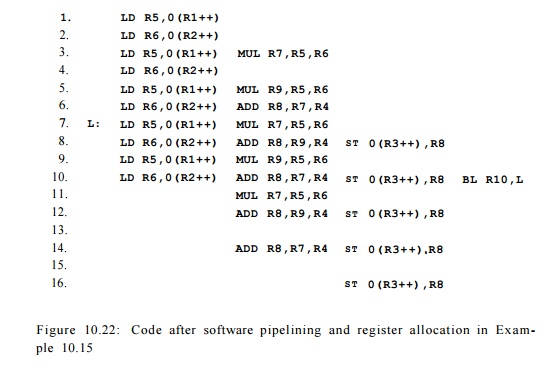
To handle loops that have fewer than 5 iterations and loops with an even number of iterations, we generate the code whose source-level equivalent is shown in Fig. 10.21. The first loop is pipelined, as seen in the machine-level equivalent of Fig. 10.22. The second loop of Fig. 10.21 need not be optimized, since it can iterate at most four times. •

4. Do-Across Loops

Software pipelining can also be applied to loops whose iterations share data dependences. Such loops are known as do-across loops.

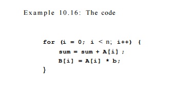
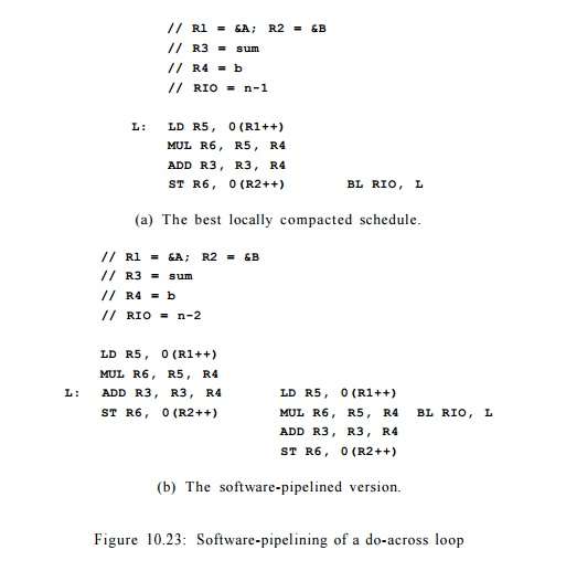
has a data dependence between consecutive iterations, because the previous value of sum is added to A[i] to create a new value of sum. It is possible to execute the summation in 0(logn) time if the machine can deliver sufficient parallelism, but for the sake of this discussion, we simply assume that all the sequential dependences must be obeyed, and that the additions must be performed in the original sequential order. Because our assumed machine model takes two clocks to complete an ADD, the loop cannot execute faster than one iteration every two clocks. Giving the machine more adders or multipliers will not make this loop run any faster. The throughput of do-across loops like this one is limited by the chain of dependences across iterations.

The best locally compacted schedule for each iteration is shown in Fig. 10.23(a), and the software-pipelined code is in Fig. 10.23(b). This software-pipelined loop starts an iteration every two clocks, and thus operates at the optimal rate.

5. Goals and Constraints of Software Pipelining

The primary goal of software pipelining is to maximize the throughput of a long-running loop. A secondary goal is to keep the size of the code generated reasonably small. In other words, the software-pipelined loop should have a small steady state of the pipeline. We can achieve a small steady state by requiring that the relative schedule of each iteration be the same, and that the iterations be initiated at a constant interval. Since the throughput of the loop is simply the inverse of the initiation interval, the objective of software pipelining is to minimize this interval.

A software-pipeline schedule for a data-dependence graph G — (N, E) can be specified by

1.    An initiation interval T and

2.    A relative schedule 5" that specifies, for each operation, when that opera-tion is executed relative to the start of the iteration to which it belongs.

Thus, an operation n in the ith iteration, counting from 0, is executed at clock i x T+S(n). Like all the other scheduling problems, software pipelining has two kinds of constraints: resources and data dependences. We discuss each kind in detail below.

Modular  Resource  Reservation

Let a machine's resources be represented by R = [ri,r2, • . . ] , where ri is the number of units of the ith kind of resource available. If an iteration of a loop requires ni units of resource i, then the average initiation interval of a pipelined loop is at least m.axi(rii/ri) clock cycles. Software pipelining requires that the initiation intervals between any pair of iterations have a constant value. Thus, the initiation interval must have at least maxi1ni/ri] clocks. If max^(rii/ri) is less than 1, it is useful to unroll the source code a small number of times.

Example 10. 17 : Let us return to our software-pipelined loop shown in Fig. 10.20. Recall that the target machine can issue one load, one arithmetic op-eration, one store, and one loop-back branch per clock. Since the loop has two loads, two arithmetic operations, and one store operation, the minimum initiation interval based on resource constraints is 2 clocks.

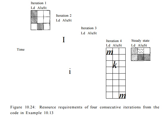
Figure 10.24 shows the resource requirements of four consecutive iterations across time. More resources are used as more iterations get initiated, culminating in maximum resource commitment in the steady state. Let RT be the resource-reservation table representing the commitment of one iteration, and let RT_S represent the commitment of the steady state. RT_S combines the commit-ment from four consecutive iterations started T clocks apart. The commitment of row 0 in the table RT$ corresponds to the sum of the resources committed in RT[0], RT[2], RT[4], and RT[6]. Similarly, the commitment of row 1 in the ta-ble corresponds to the sum of the resources committed in RT[1], RT[3], RT[h], and RT[7]. That is, the resources committed in the ith row in the steady state are given by

We refer to the resource-reservation table representing the steady state as the modular resource-reservation table of the pipelined loop.

To check if the software-pipeline schedule has any resource conflicts, we can simply check the commitment of the modular resource-reservation table. Surely, if the commitment in the steady state can be satisfied, so can the commitments in the prolog and epilog, the portions of code before and after the steady-state loop. •

In general, given an initiation interval T and a resource-reservation table of an iteration RT, the pipelined schedule has no resource conflicts on a machine with resource vector R if and only if RTs[i] < R for all* = 0 , 1 , . . . , T — 1.

Data - Dependence  Constraints

Data dependences in software pipelining are different from those we have en-countered so far because they can form cycles. An operation may depend on the result of the same operation from a previous iteration. It is no longer ade-quate to label a dependence edge by just the delay; we also need to distinguish between instances of the same operation in different iterations. We label a de-pendence edge ni -»• n₂ with label (8, d) if operation n₂ in iteration i must be delayed by at least d clocks after the execution of operation n1 in iteration i — 8. Let S, a function from the nodes of the data-dependence graph to integers, be the software pipeline schedule, and let T be the initiation interval target. Then

The iteration difference, 8, must be nonnegative. Moreover, given a cycle of data-dependence edges, at least one of the edges has a positive iteration differ-ence.

Example 10.18 : Consider the following loop,  and suppose we do not know the values of p and q: 

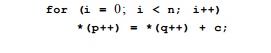
We must assume that  any pair of *(p++) and  *(q++)  accesses may refer to the same memory location. Thus, all the reads and writes must  execute in the original sequential order. Assuming that the target machine has the same characteristics as that described in Example 10.13, the data-dependence edges for this code are as shown in Fig. 10.25. Note, however, that we ignore the loop-control instructions that would have to be present, either computing and testing i, or doing the test based on the value of Rl or R2.

The iteration difference between related operations can be greater than one, as shown in the following example:

Here the value written in iteration i is used two iterations later. The dependence edge between the store of A[i] and the load of A[i — 2] thus has a difference of 2 iterations.

The presence of data-dependence cycles in a loop imposes yet another limit on its execution throughput. For example, the data-dependence cycle in Fig. 10.25 imposes a delay of 4 clock ticks between load operations from consecutive iterations. That is, loops cannot execute at a rate faster than one iteration every 4 clocks.

The initiation interval of a pipelined loop is no smaller than

clocks.

In summary, the initiation interval of each software-pipelined loop is bound-ed by the resource usage in each iteration. Namely, the initiation interval must be no smaller than the ratio of units needed of each resource and the units available on the machine. In addition, if the loops have data-dependence cycles, then the initiation interval is further constrained by the sum of the delays in the cycle divided by the sum of the iteration differences. The largest of these quantities defines a lower bound on the initiation interval.

6. A Software-Pipelining Algorithm

The goal of software pipelining is to find a schedule with the smallest possible initiation interval. The problem is NP-complete, and can be formulated as an integer-linear-programming problem. We have shown that if we know what the minimum initiation interval is, the scheduling algorithm can avoid resource con-flicts by using the modular resource-reservation table in placing each operation. But we do not know what the minimum initiation interval is until we can find a schedule. How do we resolve this circularity?

We know that the initiation interval must be greater than the bound com-puted from a loop's resource requirement and dependence cycles as discussed above. If we can find a schedule meeting this bound, we have found the opti-mal schedule. If we fail to find such a schedule, we can try again with larger initiation intervals until a schedule is found. Note that if heuristics, rather than exhaustive search, are used, this process may not find the optimal schedule.

Whether we can find a schedule near the lower bound depends on properties of the data-dependence graph and the architecture of the target machine. We can easily find the optimal schedule if the dependence graph is acyclic and if every machine instruction needs only one unit of one resource. It is also easy to find a schedule close to the lower bound if there are more hardware resources than can be used by graphs with dependence cycles. For such cases, it is advisable to start with the lower bound as the initial initiation-interval target, then keep increasing the target by just one clock with each scheduling attempt . Another possibility is to find the initiation interval using a binary search. We can use as an upper bound on the initiation interval the length of the schedule for one iteration produced by list scheduling.