Graphing Functions using Transformations

Graphing Functions using Transformations

“A picture is worth a thousand words” is a well known proverb. To know about a function well, its graph will help us more than its analytical expression. To draw graphs quickly without plotting many points is an invaluable skill. Familiarity with shapes of some basic functions will help to graph other complicated functions. Understanding and usage of symmetry and transformations will then enable to strengthen graphing abilities. This section is not simply a data base of graphs, we learn some methods to graph certain functions.

Suppose that we want to draw or sketch the curve of the function y = 2 sin(x − 1) + 3. At the very first sight it looks that it is very difficult to draw the curve representing this function. But it will be very easy to draw after understanding the content of this section.

If we know a half of a graph is the mirror image of the other half with respective to a line, or a graph can be obtained just by moving a known graph in some direction, then we can draw the new one using the known one. Moreover if we know that a graph can be obtained by enlarging or shrinking a known one, then also we can draw the new one using the known ones.

The following type of transformations play very important roles in graphing.

i.            Reflection

ii.            Translation

iii.            Dilations.

In the case of reflections and translations, they produce graphs congruent to the original graph; that is, the size and the shape of the graph does not change, but in dilation, it produce graphs with shapes related to those of the original graph.

Reflection

The reflection of the graph of a function with respect to a line is the graph that is symmetric to it with respect to . A reflection is the mirror image of the graph where line is the mirror of the reflection. (See Figure 1.47.)

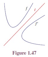
Here f ‘ is the mirror image of f with respect to . Every point of f has a corresponding image in f’ . Some useful reflections of y = f(x) are

i.            The graph y = −f(x) is the reflection of the graph of f about the x-axis.

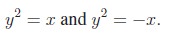
ii.            The graph y = f(−x) is the reflection of the graph of f about the y-axis.

iii.            The graph of y = f⁻¹(x) is the reflection of the graph of f in y = x.

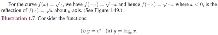
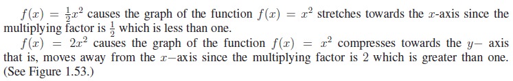
Illustration 1.5  Consider the functions:

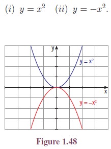
For the curve f(x) = x², −f(x) = −x². Hence, y = −x² is the reflection of y = x² about x-axis. (See Figure 1.48.)

Illustration 1.6  Consider the positive branches of

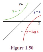
We know that, y = e^x is the inverse function of y = log_e x and hence y = e^x is the reflection of

= log_e x about y = x. (See Figure 1.50.)

Translation

A translation of a graph is a vertical or horizontal shift of the graph that produces congruent graphs.

The graph of

y = f(x + c),c> 0 causes the shift to the left.

y = f(x − c),c> 0 causes the shift to the right.

y = f(x) + d, d > 0 causes the shift to the upward.

y = f(x) − d, d > 0 causes the shift to the downward.

Illustration 1.8 Consider the functions:

f(x) = |x| (ii) f(x) = |x − 1| (iii) f(x) = |x + 1|

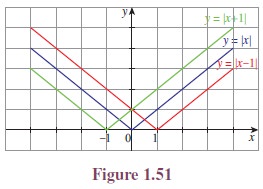
f(x) = |x − 1| causes the graph of the function f(x) = |x| shifts to the right for one unit.

f(x) = |x + 1| causes the graph of the function f(x) = |x| shifts to the left for one unit.

(See Figure 1.51.)

Illustration 1.9 Consider the functions:

(i) f(x) = |x| (ii) f(x) = |x| − 1 (iii) f(x) = |x| + 1

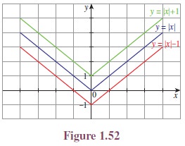
f(x) = |x| − 1 causes the graph of the functionf(x) = |x| shifts to the downward for one unit.

f(x) = |x| + 1 causes the graph of the function f(x) = |x| shifts to the upward for one unit. (See Figure 1.52.)

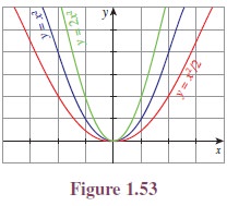
Dilation

Dilation is also a transformation which causes the curve stretches (expands) or compresses (con-tracts). Multiplying a function by a positive constant vertically stretches or compresses its graph; that is, the graph moves away from x-axis or towards x-axis.

If the positive constant is greater than one, the graph moves away from the x-axis. If the positive constant is less than one, the graph moves towards the x-axis.

Illustration 1.10  Consider the functions:

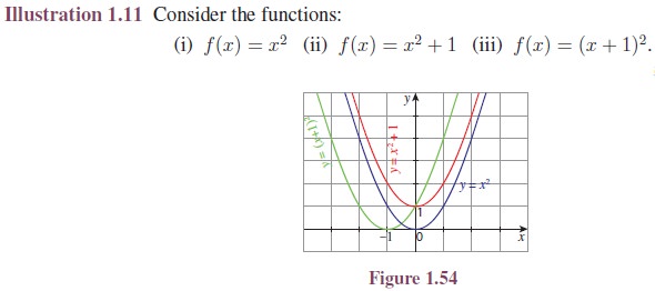
The graphs Figures 1.55 and 1.56 look identical until we compare the scales on the y-axis. The scale in Figure 1.56 is four times as large, reflecting the multiplication of the original function by 4 (Figure 1.55). The effect looks different when the functions are plotted on the same scale as in Figure 1.57.

The graph of y = (4x)² − 1 is shown in Figure 1.58. Can you spot the difference between Figure 1.55 and Figure 1.58? In this case, x-scale has now changed, by the same factor of 4 as in the function (Figure 1.58). To see this, note that substituting x = 1/4 into (4x)² − 1 produces 1² − 1, exactly the same as substituting x = 1 into the original function (Figure 1.55). When plotted on the same set of axes (as in Figure 1.59) the parabola y = (4x)² − 1 looks thinner. Here, the x-intercepts are different, but y-intercepts are the same.

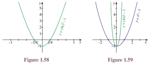
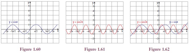
Illustration 1.13  By using the same concept applied in Illustration 1.12, graphs of y = sin x and y= sin 2x, and also their combined graphs are given Figures 1.60, 1.61 and 1.62. The minimum and maximum values of sin x and sin 2x are the same. But they have different x-intercepts. The x-intercepts for y = sin x are ±nπ and for y = sin 2x are ±1/2 nπ, n ∈ Z.

In the beginning of the section we talked about drawing the graph of y = 2 sin(x − 1) + 3. Now we are well equipped to draw the curve and even we can draw more complicated curve.

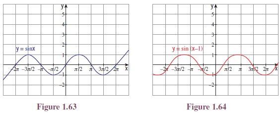
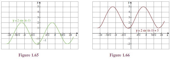
Illustration 1.14  Let us now draw the graph of y = 2 sin(x − 1) + 3.

It is clear that the curve can be obtained from that of y = sin x using translation and dilation.

So first we draw y = sin x. From that it is easy to draw the curve y = sin(x − 1); then draw y = 2 sin(x − 1) and finally y = 2 sin(x − 1) + 3. (See Figures 1.63 to 1.66.)