Computer Graphics

PREREQUISITE DISCUSSION:

In this unit we discuss about drawing algorithms, clipping algorithms, How to find out a pixel points In between line path and circle.

1. SURVEY OF COMPUTER GRAPHICS, OVERVIEW OF GRAPHICS SYSTEMS :

CONCEPT:

1.Applications

2.Interaction to the real world

3.CAD/CAM

4.Videos,Musics

A picture is completely specified by the set of intensities for the pixel positions inthe display. Shapes and colors of the objects can be described internally with pixelarrays into the frame buffer or with the set of the basic geometric – structure such asstraight line segments and polygon color areas. To describe structure of basic objectis referred to as output primitives.Each output primitive is specified with input co-ordinate data and other information about the way that objects is to be displayed. Additional output primitives that canbe used to constant a picture include circles and other conic sections, quadric surfaces, Spline curves and surfaces, polygon floor areas and character string.

SIGNIFICANCE:

It is important to real world entertainment activities and medical fields

2.VIDEO DISPLAY DEVICES, RASTER SCANSYSTEMS, RANDOM SCAN SYSTEMS, GRAPHICS MONITORS AND WORKSTATIONS,INPUT DEVICES, HARD COPYDEVICES, GRAPHICS SOFTWARE

CONCEPT:

Video display devices:

1.Primary output device

2.Used Cathode Ray tubes

3.Electrons emmitted and reflected.

Raster Scansystems, Random Scan Systems:

1.Afixed area of the system

2.Video controller is given direct access in frame buffered.

3.The coordinate origin is defined at the lower left screen corner.

Graphics Monitors And Workstations

1.Diagonal screen dimensions

2.12 to 2 inches

3.High definition graphics monitors

Input Devices & Hard Copy devices

1.Key board 2.Pen light 3.Joy sticks 4.Touch panels 5.Digitizers

* Printers

Impact printers

Non Impact printers

3. OUTPUT PRIMITIVES

CONCEPT:

A picture is completely specified by the set of intensities for the pixel positions in the display. Shapes and colors of the objects can be described internally with pixel arrays into the frame buffer or with the set of the basic geometric – structure such as straight line segments and polygon color areas. To describe structure of basic object is referred to as output primitives. Each output primitive is specified with input co-ordinate data and other information about the way that objects is to be displayed. Additional output primitives that can be used to constant a picture include circles and other conic sections, quadric surfaces, Spline curves and surfaces, polygon floor areas and character string.

4. POINTS AND LINES POINT PLOTTING

CONCEPT

It is accomplished by converting a single coordinate position furnished by an application program into appropriate operations for the output device.

With a CRT monitor, for example, the electron beam is turned on to illuminate the screen phosphor at the selected location Line drawing is accomplished by calculating intermediate positions along the line path between two specified end points positions. An output device is then directed to fill in these positions between the end points Digital devices display a straight line segment by plotting discrete points between the two end points. Discrete coordinate positions along the line path are calculated from the equation of the line.

For a raster video display, the line color (intensity) is then loaded into the frame buffer at the corresponding pixel coordinates. Reading from the frame buffer, the video controller then plots “the screen pixels”. Pixel positions are referenced according to scan-line number and column number (pixel

position across a scan line).

Scan lines are numbered consecutively from 0, starting at the bottom of the screen; and pixel columns are numbered from 0, left to right across each scan line Figure : Pixel Postions reference by scan line number and column number To load an intensity value into the frame buffer at a position corresponding to column x along scan line y, setpixel (x, y) To retrieve the current frame buffer intensity setting for a specified location we use a low level function getpixel (x, y)

SIGNIFICANCE:

It is used to plot the points and lines within the coordinates.

LINE DRAWING ALGORITHMS

CONCEPT:

·     Digital Differential Analyzer (DDA) Algorithm

·     Bresenham  s Line Algorithm

·     Parallel Line Algorithm

The Cartesian slope-intercept equation for a straight line is y = m . x + b (1) Where m as slope of the line and b as the y intercept

(x2,y2) as in figure we can determine the values for the slope m and y intercept b with the following calculations

Line Path between endpoint positions (x1,y1) and (x2,y2)

m = Δy / Δx = y2-y1 / x2 - x1 (2)

b= y1 - m . x1 (3) For any given x interval Δx along a line, we can compute the corresponding y interval y Δy= m Δx (4) We can obtain the x interval Δx corresponding to a specified Δy as   x =   y/m (5) For lines with slope magnitudes |m| < 1, Δx can be set proportional to a small horizontal deflection voltage and the corresponding vertical deflection is then set proportional to Δy as calculated from Eq (4). For lines whose slopes have magnitudes |m | >1 , Δy can be set proportional to a small vertical deflection voltage with the corresponding horizontal deflection voltage set proportional to Δx, calculated from Eq

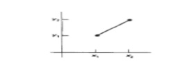
(5) For lines with m = 1, Δx = Δy and the horizontal and vertical deflections voltage are equal. Figure :

Straight line Segment with five sampling positions along the x axis between x1 and x2

Digital Differential Analyzer (DDA) Algortihm

The digital differential analyzer (DDA) is a scan-conversion line algorithm based on calculation either Δy or Δx The line at unit intervals in one coordinate and determine corresponding integer values

nearest the line path for the other coordinate.

A line with positive slop, if the slope is less than or equal to 1, at unit x intervals (Δx=1) and compute each successive y values as yk+1 = yk + m (6) Subscript k takes integer values starting from 1 for the first point and increases by 1 until the final endpoint is reached. m can be any real number

between 0 and 1 and, the calculated y values must be rounded to the nearest integer For lines with a positive slope greater than 1 we reverse the roles of x and y, (Δy=1) and calculate each succeeding x

value as xk+1 = xk + (1/m) (7) Equation (6) and (7) are based on the assumption that lines are to be processed from the left endpoint to the right endpoint.

If this processing is reversed, Δx=-1 that the starting endpoint is at the right yk+1 = yk – m (8) When the slope is greater than 1 and Δy = -1 with xk+1 = xk-1(1/m) (9) If the absolute value of the slope is less than 1 and the start endpoint is at the left, we set Δx = 1 and calculate y values with Eq. (6) When the start endpoint is at the right (for the same slope), we set Δx = -1 and obtain y positions from Eq. (8) . Similarly, when the absolute value of a negative slope is greater than 1, we use Δy = -1 and Eq. (9) or we use Δy = 1

and Eq. (7).

Algorithm

#define ROUND(a) ((int)(a+0.5))

void lineDDA

(int xa, int ya, int xb, int yb)

{ int dx = xb - xa, dy = yb - ya, steps, k; float xIncrement, yIncrement, x = xa, y = ya; if (abs (dx) > abs (dy) steps = abs (dx) ; else steps = abs dy); xIncrement = dx / (float) steps; yIncrement = dy / (float) steps setpixel (ROUND(x), ROUND(y) ) : for (k=0; k<steps; k++)

{ x += xIncrement; y += yIncrement; setpixel (ROUND(x), ROUND(y)); } } Algorithm Description: Step 1 : Accept Input as two endpoint pixel positions

Step 2: Horizontal and vertical differences between the endpoint positions are assigned to parameters dx and dy (Calculate dx=xb-xa and dy=yb-ya).

Step 3: The difference with the greater magnitude determines the value of parameter steps.

Step 4 : Starting with pixel position (xa, ya), determine the offset needed at each step to generate the next pixel position along the line path.

Step 5: loop the following process for steps number of times

a.                 Use a unit of increment or decrement in the x and y direction

b.if xa is less than xb the values of increment in the x and y directions are 1 and m

c.if xa is greater than xb then the decrements -1 and – m are used.

Advantages of DDA Algorithm

1.     It is the simplest algorithm

2. It is a is a faster method for calculating pixel positions

Disadvantages of DDA Algorithm

1.Floating point arithmetic in DDA algorithm is still time-consuming

2.End point accuracy is poor

Bresenham’s Line Algorithm

An accurate and efficient raster line generating algorithm developed by Bresenham, that uses only incremental integer calculations. In addition, Bresenhams line algorithm can be adapted to display circles and other curves. To illustrate Bresenham's approach, we- first consider the scan-conversion process for lines with positive slope less than 1. Pixel positions along a line path are then determined by sampling at unit x intervals. Starting from the left endpoint (x0,y0) of a given line, we step to each successive column (x position) and plot the pixel whose scan-line y value is closest to the line path.

To determine the pixel (xk,yk) is to be displayed, next to decide which pixel to plot the column xk+1=xk+1.(xk+1,yk) and .(xk+1,yk+1).

At sampling position xk+1, we label vertical pixel separations from the mathematical line path as d1 and d2. The y coordinate on the mathematical line at pixel column position xk+1 is calculated as y =m(xk+1)+b (1) Then d1 = y-yk = m(xk+1)+b-yk d2 = (yk+1)-y = yk+1-m(xk+1)-b To determine which of the two pixel is closest to the line path, efficient test that is based on the difference between the two pixel separations d1- d2 = 2m(xk+1)-2yk+2b-1 (2) A decision parameter Pk for the kth step in the line algorithm can be obtained by rearranging equation (2).

By substituting m=Δy/Δx where Δx and Δy are the vertical and horizontal separations of the endpoint positions and defining the decision parameter as pk = Δx (d1- d2) = 2Δy xk.-2Δx. yk + c (3) The sign of pk is the same as the sign of d1- d2,since Δx>0

Parameter C is constant and has the value 2Δy + Δx(2b -1) which is independent of the pixel position and will be eliminated in the recursive calculations for Pk. If the pixel at yk is “closer” to the line

path than the pixel at yk+1 (d1< d2) than decision parameter Pk is negative.

In this case, plot the lower pixel, otherwise plot the upper pixel. Coordinate changes along the line occur in unit steps in either the x or y directions. To obtain the values of successive decision parameters using incremental integer calculations.

At steps k+1, the decision parameter is evaluated from equation (3) as Pk+1 = 2Δy xk+1-2Δx. yk+1 +c Subtracting the equation (3) from the preceding equation Pk+1 - Pk = 2Δy (xk+1 - xk) -

2Δx(yk+1 - yk) But xk+1= xk+1 so that Pk+1 = Pk+ 2Δy-2Δx(yk+1 - yk) (4) Where the term yk+1-yk is either 0 or 1 depending on the sign of parameter Pk

This recursive calculation of decision parameter is performed at each integer x position, starting

at the left coordinate endpoint of the line. The first parameter P0 is evaluated from equation at the starting pixel position (x0,y0) and with m evaluated as Δy/Δx P0 = 2Δy-Δx (5) Bresenham s line drawing for a line with a positive slope less than 1 in the following outline of the algorithm. The constants 2Δy and2Δy-2Δx are calculated once for each line to be scan converted. Bresenham’s line Drawing Algorithm for |m| < 1

1.Input the two line endpoints and store the left end point in (x0,y0)

2.load (x0,y0) into frame buffer, ie. Plot the first point.

3. Calculate the constants Δx, Δy, 2Δy and obtain the starting value for the decision parameter as P0 = 2Δy-Δx

4.At each xk along the line, starting at k=0 perform the following test

If Pk < 0, the next point to plot is(xk+1,yk) and Pk+1 = Pk + 2Δy otherwise, the next point to plot is (xk+1,yk+1) and Pk+1 = Pk + 2Δy - 2Δx 5. Perform step4 Δx times.

Implementation of Bresenham Line drawing Algorithm

void lineBres (int xa,int ya,int xb, int yb)

{

int dx = abs( xa – xb) , dy = abs (ya - yb); int p = 2 * dy – dx; int twoDy = 2 * dy, twoDyDx = 2 *(dy - dx);

int x , y, xEnd; /* Determine which point to use as start, which as end * / if (xa > x b ) { x = xb; y = yb; xEnd = xa; }

else { x = xa; y = ya; xEnd = xb; }

setPixel(x,y); while(x<xEnd) { x++; if (p<0) p+=twoDy; { y++; p+=twoDyDx;

}

setPixel(x,y);

}

}

Advantages

Algorithm is Fast

Uses only integer calculations

Disadvantages

It is meant only for basic line drawing.

Circle-Generating Algorithms

General function is available in a graphics library for displaying various kinds of curves, including circles and ellipses.

Properties of a circle

A circle is defined as a set of points that are all the given distance (xc,yc). This distance relationship is expressed by the pythagorean theorem in Cartesian coordinates as

(x – xc)2 + (y – yc) 2 = r2 (1) Use above equation to calculate the position of points on a circle circumference by stepping along the x axis in unit steps from xc-r to xc+r and calculating the corresponding y values at each position as y = yc +(- ) (r2 – (xc –x )2)1/2 (2) This is not the best method for generating a circle for the following reason Considerable amount

of computation Spacing between plotted pixels is not uniform To eliminate the unequal spacing is to calculate points along the circle boundary using polar coordinates r and θ.

Expressing the circle equation in parametric polar from yields the pair of equations x = xc + rcos θ y = yc + rsin θ When a display is generated with these equations using a fixed angular step size, a circle

is plotted with equally spaced points along the circumference.

To reduce calculations use a large angular separation between points along the circumference and connect the points with straight line segments to approximate the circular path. Set the angular step size at 1/r. This plots pixel positions that are approximately one unit apart. The shape of the circle is similar in each quadrant.

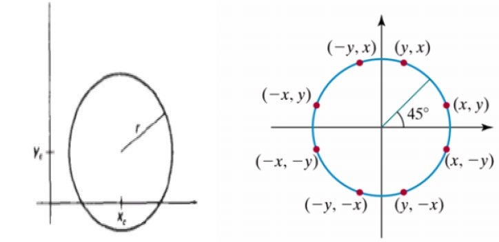
To determine the curve positions in the first quadrant, to generate he circle section in the second quadrant of the xy plane by nothing that the two circle sections are symmetric with respect to the y axis and circle section in the third and fourth quadrants can be obtained from sections in the first and second quadrants by considering symmetry between octants.

\

Circle sections in adjacent octants within one quadrant are symmetric with respect to the 450 line dividing the two octants. Where a point at position (x, y) on a one-eight circle sector is mapped into the seven circle points in the other octants of the xy plane.

To generate all pixel positions around a circle by calculating only the points within the sector from x=0 to y=0. the slope of the curve in this octant has an magnitude less than of equal to 1.0. at x=0, the circle slope is 0 and at x=y, the slope is -1.0.

Midpoint circle Algorithm:

In the raster line algorithm at unit intervals and determine the closest pixel position to the specified circle path at each step for a given radius r and screen center position (xc,yc) set up our algorithm to calculate pixel positions around a circle path centered at the coordinate position by adding xc to x and yc to y.

To apply the midpoint method we define a circle function as fcircle(x,y) = x2+y2-r2 Any point (x,y) on the boundary of the circle with radius r satisfies the equation fcircle (x,y)=0. If the point is in the interior of the circle, the circle function is negative. And if the point is outside the circle the, circle function is positive fcircle (x,y) <0, if (x,y) is inside the circle boundary =0, if (x,y) is on the circle boundary >0, if (x,y) is outside the circle boundary

The tests in the above eqn are performed for the midposition sbteween pixels near the circle path at each sampling step. The circle function is the decision parameter in the midpoint algorithm.

.Ellipse-Generating Algorithms

An ellipse is an elongated circle. Therefore, elliptical curves can be generated by modifying circle-drawing procedures to take into account the different dimensions of an ellipse along the major and minor axes.

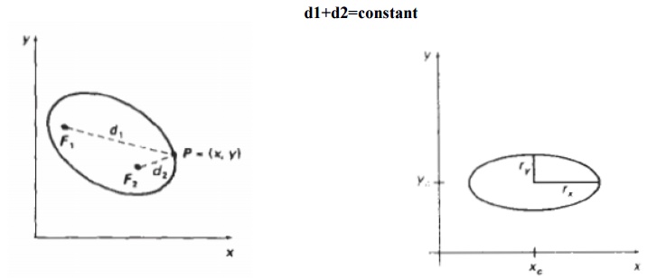
Properties of ellipses

An ellipse can be given in terms of the distances from any point on the ellipse to two fixed positions called the foci of the ellipse. The sum of these two distances is the same values for all points on the ellipse. If the distances to the two focus positions from any point p=(x,y) on the ellipse are labeled d1 and d2, then the general equation of an ellipse can be stated as

d1+d2=constant

Midpoint ellipse Algorithm

The midpoint ellipse method is applied throughout the first quadrant in two parts. The below figure show the division of the first quadrant according to the slope of an ellipse with rx<ry. In the x direction where the slope of the curve has a magnitude less than 1 and unit steps in the y direction where the slope has a magnitude greater than 1. Region 1 and 2 can be processed in various ways

1. Start at position (0,ry) and step clockwise along the elliptical path in the first quadrant shifting from unit steps in x to unit steps in y when the slope becomes less than -1

2. Start at (rx,0) and select points in a counter clockwise order. 2.1 Shifting from unit steps in y to unit steps in x when the slope becomes greater than -1.0 2.2 Using parallel processors calculate pixel positions in the two regions simultaneously

3. Start at (0,ry) step along the ellipse path in clockwise order throughout the first quadrant ellipse function (xc,yc)=(0,0)

fellipse (x,y)=ry2x2+rx2y2 –rx2 ry2 which has the following properties: fellipse (x,y) <0, if (x,y) is inside the ellipse boundary =0, if(x,y) is on ellipse boundary >0, if(x,y) is outside the ellipse boundary Thus, the ellipse function

fellipse (x,y) serves as the decision parameter in the midpoint algorithm. Starting at (0,ry): Unit steps in the x direction until to reach the boundary between region 1 and region 2. Then switch to unit steps in the y direction over the remainder of the curve in the first quadrant. At each step to test the value of the slope of the curve. The ellipse slope is calculated dy/dx= -(2ry2x/2rx2y) At the boundary between region 1 and region 2 dy/dx = -1.0 and 2ry2x=2rx2y to more out of region 1 whenever 2ry2x>=2rx2y

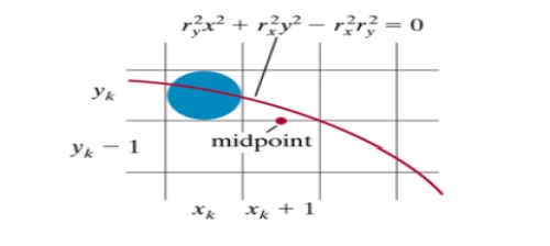
To determine the next position along the ellipse path by evaluating the decision parameter at this mid point P1k = fellipse (xk+1,yk-1/2) = ry2 (xk+1)2 + rx2 (yk-1/2)2 – rx2 ry2 if P1k <0,

The midpoint is inside the ellipse and the pixel on scan line yk is closer to the ellipse boundary. Otherwise the midpoint is outside or on the ellipse boundary and select the pixel on scan line yk-1 At the next sampling position (xk+1+1=xk+2) the decision parameter for region 1 is calculated as p1k+1 = fellipse(xk+1 +1,yk+1 -½ ) =ry2[(xk +1) + 1]2 + rx2 (yk+1 -½)2 - rx2 ry2

Mid point Ellipse Algorithm

1. Input rx,ry and ellipse center (xc,yc) and obtain the first point on an ellipse centered on the origin as

(x0,y0) = (0,ry)

2. Calculate the initial value of the decision parameter in region 1 as

P10=ry2-rx2ry +(1/4)rx2

3. At each xk position in region1 starting at k=0 perform the following test. If P1k<0, the next point along the ellipse centered on (0,0) is (xk+1, yk) and

p1k+1 = p1k +2 ry2xk +1 + ry2 Otherwise the next point along the ellipse is (xk+1, yk-1) and p1k+1 = p1k +2 ry2xk +1 - 2rx2 yk+1 + ry2 with 2 ry2xk +1 = 2 ry2xk + 2ry2 2 rx2yk +1 = 2 rx2yk + 2rx2 And continue until 2ry2 x>=2rx2 y

4. Calculate the initial value of the decision parameter in region 2 using the last point (x0,y0) is the last position calculated in region 1.

p20 = ry2(x0+1/2)2+rx2(yo-1)2 – rx2ry2

5. At each position yk in region 2, starting at k=0 perform the following test, If p2k>0 the next point along the ellipse centered on (0,0) is (xk,yk-1) and

p2k+1 = p2k – 2rx2yk+1+rx2 Otherwise the next point along the ellipse is (xk+1,yk-1) and

p2k+1 = p2k + 2ry2xk+1 – 2rxx2yk+1 + rx2 Using the same incremental calculations for x any y as in region 1.

7.  6. Determine symmetry points in the other three quadrants. Move each calculate pixel position (x,y) onto the elliptical path centered on (xc,yc) and plot the coordinate values

x=x+xc, y=y+yc

8.Repeat the steps for region1 unit 2ry2x>=2rx2y

SIGNIFICANCE:

Draw a circle ,lines and ellipse using Differant types of algorithms.

Line function

Any parameter that affects the way a primitive is to be displayed is referred to as an attribute parameter.

1.Line Attributes

2.Curve Attributes

3.Color and Grayscale Levels

4.Area Fill Attributes

5.Character Attributes

6.Bundled Attributes

Line Attributes

Basic attributes of a straight line segment are its type, its width, and its color. In some graphics packages, lines can also be displayed using selected pen or brush options

Line Type

Line Width

Pen and Brush Options Line Color

Line type

Possible selection of line type attribute includes solid lines, dashed lines and dotted lines. To set line type attributes in a PHIGS application program, a user invokes the function

setLinetype (lt)

Line width

Implementation of line width option depends on the capabilities of the output device to set the line width attributes.

setLinewidthScaleFactor(lw)

Line Cap

We can adjust the shape of the line ends to give them a better appearance by adding line caps. There are three types of line cap. They are

Butt cap

Round cap

Projecting square cap

Pen and Brush Options

With some packages, lines can be displayed with pen or brush selections. Options in this category include shape, size, and pattern. Some possible pen or brush shapes

setPolylineColourIndex (lc)

Curve attributes

Parameters for curve attribute are same as those for line segments. Curves displayed with varying colors, widths, dot –dash patterns and available pen or brush options

Area fill Attributes

Options for filling a defined region include a choice between a solid color or a pattern fill and choices for particular colors and patterns Fill Styles Areas are displayed with three basic fill styles: hollow with a color border, filled with a solid color, or filled with a specified pattern or design. A basic fill style is selected in a PHIGS program with the function

Character Attributes

The appearance of displayed character is controlled by attributes such as font, size, color and orientation. Attributes can be set both for entire character strings (text) and for individual characters defined as marker symbols

Text Attributes

The choice of font or type face is set of characters with a particular design style as courier, Helvetica, times roman, and various symbol groups.

SIGNIFICANCE:

Different types of functions used to implement line circle.

5. PIXEL ADDRESSING AND OBJECTGEOMETRY

CONCEPT:

1.Pixel Value Is An Intensity Value It Is Stored In Frame Buffered

2.Particular All Images Are Descibed In Pixels.

SIGNIFICANCE:

It is used to stored a pixel value in the frame buffer

6. FILLED AREA PRIMITIVES

1.Set the width of line-clipping 

2.Set color of particular pictures

APPLICATIONS:

1Implement. Line,circle,ellipse drawing algorithm. 

2.Importance of CRT monitors

3.Implement loading the frame buffer.