Chapter: Computer Graphics and Architecture
Animations & Realism
ANIMATIONS
& REALISM
PREREQUISITE DISCUSSION:
This unit give brief explanation about fractals, Peanocurves,
and ray tracing
1. ANIMATION
CONCEPT :
Computer animation refers to any time
sequence of visual changes in a scene.
Computer
animations can also be generated by changing camera parameters such as
position, orientation and focal length.
Applications of computer-generated
animation are entertainment, advertising, training and education.
Example :
Advertising animations often transition one object shape into
another. Frame-by-Frame animation Each frame of the scene is separately
generated and stored. Later, the frames can be recoded on film or they
can be consecutively displayed in "real-time playback" mode Design
of Animation Sequences An animation sequence in designed with the
following steps:
Story board layout
Object definitions
Key-frame specifications
Generation of in-between frames.
Story board
The story board is an outline of the
action.
It defines the motion sequences as a
set of basic events that are to take place.
Depending
on the type of animation to be produced, the story board could consist of a set
of rough sketches or a list of the basic ideas for the motion.
Object Definition
An object definition is given for each
participant in the action.
Objects can be defined in terms of
basic shapes such as polygons or splines.
The associated movements of each
object are specified along with the shape.
SIGNIFICANCE:
Computer animation refers to any time sequence of visual changes
in a scene.
2. KEY
FRAME
CONCEPT
A key frame is detailed drawing of the
scene at a certain time in the animation sequence.
Within each key frame, each object is
positioned according to the time for that frame.
Some key
frames are chosen at extreme positions in the action; others are spaced so that
the time interval between key frames is not too much.
3. Computer Animation
Languages
Animation functions include a graphics editor, a key
frame generator and standard graphics routines.
The graphics editor
allows designing and modifying object shapes, using spline surfaces,
constructive solid geometry methods or other representation schemes.
Scene description
includes the positioning of objects and light sources defining the photometric
parameters and setting the camera parameters.
Action specification involves the layout of motion
paths for the objects and camera.
Keyframe systems are
specialized animation languages designed dimply to generate the in-betweens
from the user specified keyframes.
Parameterized systems
allow object motion characteristics to be specified as part of the object
definitions. The adjustable parameters control such object characteristics as
degrees of freedom motion limitations and allowable shape changes.
Scripting systems allow
object specifications and animation sequences to be defined with a user input
script. From the script, a library of various objects and motions can be
constructed.
Keyframe Systems
Each set of in-betweens are generated from the
specification of two keyframes.
For complex scenes, we
can separate the frames into individual components or objects called cells, an
acronym from cartoon animation.
4. MORPHING
Transformation of object shapes from one form to
another is called Morphing.
Morphing methods can be
applied to any motion or transition involving a change in shape. The example is
shown in the below figure.
The general
preprocessing rules for equalizing keyframes in terms of either the number of
vertices to be added to a keyframe.
Suppose we equalize the
edge count and parameters Lk and Lk+1 denote the number of line segments in two
consecutive frames. We define,
Lmax = max (Lk, Lk+1)
Lmin = min(Lk , Lk+1) Ne = Lmax mod Lmin Ns = int (Lmax/Lmin) The preprocessing
is accomplished by
1.Dividing
Ne edges of keyframemin into Ns+1 section.
2.Dividing
the remaining lines of keyframemin into Ns sections.
For example, if Lk = 15
and Lk+1 = 11, we divide 4 lines of keyframek+1 into 2 sections each. The
remaining lines of keyframek+1 are left infact.
If the vector counts in
equalized parameters Vk and Vk+1 are used to denote the number of vertices in
the two consecutive frames. In this case we define
Vmax = max(Vk,Vk+1), Vmin = min( Vk,Vk+1) and Nls =
(Vmax -1) mod (Vmin – 1) Np = int ((Vmax
– 1)/(Vmin – 1 ))
Preprocessing using vertex count is performed by
1.Adding
Np points to Nls line section of keyframemin.
2.Adding
Np-1 points to the remaining edges of keyframemin.
Simulating Accelerations
Curve-fitting
techniques are often used to specify the animation paths between key frames.
Given the vertex positions at the key frames, we can fit the positions with
linear or nonlinear paths. Figure illustrates a nonlinear fit of key-frame
positions. This determines the trajectories for the in-betweens. To simulate
accelerations, we can adjust the time spacing for the in-betweens.
Goal Directed Systems
We can specify the motions that are to take place in
general terms that abstractly describe the actions.
These systems are
called goal directed. Because they determine specific motion parameters given
the goals of the animation.
Eg., To specify an object to „walk![]() or to „run
or to „run![]() to a particular distance.
to a particular distance.
Kinematics and Dynamics
With a kinematics
description, we specify the animation by motion parameters (position, velocity
and acceleration) without reference to the forces that cause the motion.
For constant velocity
(zero acceleration) we designate the motions of rigid bodies in a scene by
giving an initial position and velocity vector for each object.
We can specify
accelerations (rate of change of velocity ), speed up, slow downs and curved
motion paths.
An alternative approach
is to use inverse kinematics; where the initial and final positions of the
object are specified at specified times and the motion parameters are computed
by the system.
SIGNIFICANCE:
Transformation of object shapes from one form to another
5. GRAPHICS
PROGRAMMING USING OPENGL
CONCEPT:
OpenGL is a software
interface that allows you to access the graphics hardware without taking care
of the hardware details or which graphics adapter is in the system.
OpenGL is a low-level
graphics library specification. It makes available to the programmer a small
set of geomteric primitives - points, lines, polygons, images, and bitmaps.
OpenGL provides a set
of commands that allow the specification of geometric objects in two or three
dimensions, using the provided primitives, together with commands that control
how these objects are rendered (drawn).
Libraries
OpenGL Utility Library
(GLU) contains several routines that use lower-level OpenGL commands to perform
such tasks as setting up matrices for specific viewing orientations and projections
and rendering surfaces.
OpenGL Utility Toolkit
(GLUT) is a window-system-independent toolkit, written by Mark Kilgard, to hide
the complexities of differing window APIs.
6. BASIC GRAPHICS
PRIMITIVES
CONCEPTS:
OpenGL Provides tools
for drawing all the output primitives such as points, lines, triangles,
polygons, quads etc and it is defined by one or more vertices.
To draw such objects in
OpenGL we pass it a list of vertices. The list occurs between the two OpenGL
function calls glBegin() and glEnd(). The argument of glBegin() determine which
object is drawn.
These functions are
glBegin(int mode); glEnd( void ); The parameter mode of the function glBegin
can be one of the following:
GL_POINTS GL_LINES
GL_LINE_STRIP GL_LINE_LOOP
GL_TRIANGLES
GL_TRIANGLE_STRIP
GL_TRIANGLE_FAN GL_QUADS
glFlush() :
ensures
that the drawing commands are actually executed rather than stored in a buffer
awaiting (ie) Force all issued OpenGL commands to be executed
glMatrixMode(GL_PROJECTION)
: For orthographic projection
glLoadIdentity() : To load
identity matrix
SIGNIFICANCE:
Different types of graphics OPENGL functions are used to implement line,polygon.
7. FRACTALS
AND SELF-SIMILARITY
CONCEPTS:
Many of
the curves and pictures have a particularly important property called self-similar.
This means that they appear the same at every scale: No matter how much one
enlarges a picture of the curve, it has the same level of detail. Some curves
are exactly self-similar, whereby if a region is enlarged the
enlargement
looks exactly like the original. Other curves are statistically self-similar,
such that the wiggles and irregularities in the curve are the same “on the
average”, no matter how many times the
picture is enlarged. Example:
Coastline.
Successive Refinement of
Curves
A complex
curve can be fashioned recursively by repeatedly “refining” a simple curve. The
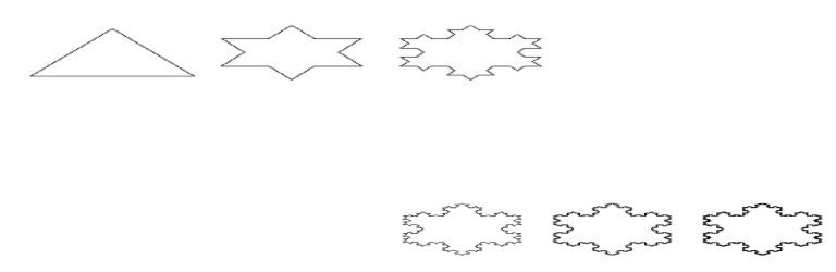
simplest example is the Koch curve, discovered in1904 by the Swedish
mathematician Helge von Koch. The curve
produces
an infinitely long line within a region of finite area. Successive generations
of the Koch curve are denoted K0, K1, K2….The zeroth generation shape K0 is a
horizontal line of length unity
To create K1 , divide
the line K0 into three equal parts and replace the middle section with a triangular
bump having sides of length 1/3. The total length of the line is 4/3. The
second order curve K2, is formed by building a bump on each of the four line
segments of K1. To form Kn+1 from Kn: Subdivide each segment of Kn into three
equal parts and replace the middle part with a bump in the shape of an
equilateral triangle.
In this process each segment is
increased in length by a factor of 4/3, so the total length of the curve is 4/3
larger than that of the previous generation. Thus Ki has total length of (4/3)i
, which increases as i increases. As i tends to infinity, the length of the
curve becomes infinite..
SIGNIFICANCE:
It gives the clear view of particular picture.
8. KOCH
CURVES
CONCEPTS:
UNDERLYING THEORY OF THE
COPYING PROCESS :
Each lens
in the copier builds an image by transforming every point in the input image
and drawing it on the output image. A black and white image I can be described
simply as the set of its black points: I = set of all black points =
{ (x,y) such that (x,y) is colored black } I is the input image to the
copier. Then the ith lens characterized by transformation Ti, builds a
new set of points we denote as Ti(I) and adds them to
the image
being produced at the current iteration. Each added set Ti(I) is the set of all
transformed points I: Ti(I) = { (x’,y’) such that (x’,y’) = Ti(P) for some
point P in I } Upon superposing the three
transformed
images, we obtain the output image as the union of the outputs from the three
lenses: Output image = T1(I) U T2(I) U T3(I) The overall mapping
from input image to output image as W(.). It maps one set of points –
one image – into another and is given by: W(.)=T1(.) U T2(.) U T3(.) For
instance the copy of the first image I0 is the set W(I0).
1.The
attractor set A is a fixed point of the mapping W(.), which we write as W(A)=A.
That is putting A through the copier again produces exactly the same image A.
The iterates have
already converged to the set A, so iterating once more makes no difference.
2.Starting
with any input image B and iterating the copying process enough times, we find
that the orbit of images always converges to the same A.
If Ik = W
(k)(B) is the kth iterate of image B, then as k goes to infinity Ik becomes
indistinguishable from the attractor A.
9. CREATING
IMAGE BY ITERATED FUNCTIONS
CONCEPTS:
Another
way to approach infinity is to apply a transformation to a picture again and
again and examine the results. This technique also provides an another method
to create fractal shapes.
An Experimental Copier
We take
an initial image I0 and put it through a special photocopier that produces a
new image I1. I1 is not a copy of I0 rather it is a superposition of several
reduced versions of I0. We then take I1 and feed it
back into the copier again, to produce
image I2. This process is repeated , obtaining a sequence of images
I0, I1, I2,… called the orbit of I0.
Making new copies from old
Underlying Theory of the Copying Process
Each lens in the copier
builds an image by transforming every point in the input image and drawing it
on the output image. A black and white image I can be described simply as the
set of its black points: I = set of all black points = { (x,y) such that
(x,y) is colored black } I is the input image to the copier. Then the ith
lens characterized by transformation Ti, builds a new set of points we denote
as Ti(I) and adds them to the image being produced at the current iteration.
Each added set Ti(I) is the set of all
transformed points
I: Ti(I) = { (x’,y’)
such that (x’,y’) = Ti(P) for some point P in I } Upon superposing the
three transformed images, we obtain the output image as the union of the
outputs from the three lenses:
Output image = T1(I) U
T2(I) U T3(I) The overall mapping from input image to
output image as W(.). It maps one set of points – one image – into
another and is given by: W(.)=T1(.) U T2(.) U T3(.) For instance the
copy of the first image I0 is the set W(I0). Each affine map reduces the size
of its image at least slightly, the orbit converge to a unique image called the
attractor of the IFS. We denote the attractor by the set A, some of its
important properties are:
1. The attractor set A
is a fixed point of the mapping W(.), which we write as W(A)=A. That is putting
A through the copier again produces exactly the same image A.
The iterates have already converged to the set A, so
iterating once more makes no difference.
2. Starting with any
input image B and iterating the copying process enough times, we find that the
orbit of images always converges to the same A.
If Ik = W
(k)(B) is the kth iterate of image B, then as k goes to infinity Ik becomes
indistinguishable from the attractor A.
Drawing the kth Iterate
We use graphics to
display each of the iterates along the orbit. The initial image I0 can be set,
but two choices are particularly suited to the tools developed:
I0 is a polyline. Then
successive iterates are collections of polylines. I0 is a single point. Then
successive iterates are collections of points.
Using a
polyline for I0 has the advantage that you can see how each polyline is reduced
in size in each successive iterate. But more memory and time are required to
draw each polyline and finally each polyline is so reduced as to be
indistinguishable from a point. Using a single point for I0 causes each iterate
to be a set of points, so it is straight forward to store these in a list. Then
if IFS consists of N affine maps, the first iterate I1 consists of N points,
image I2 consists of N2 points, I3 consists of N3 points, etc.
Copier Operation pseudocode(recursive
version)
SIGNIFICANCE:
This technique also provides an
another method to create fractal shapes.
10. THE
MANDELBROT SET
CONCEPTS:
Graphics
provides a powerful tool for studying a fascinating collection of sets that are
the most complicated objects in mathematics. Julia and Mandelbrot sets arise
from a branch of analysis known as iteration theory, which asks what happens
when one iterates a function endlessly. Mandelbrot used computer graphics to
perform experiments.
A view of
the Mandelbrot set is shown in the below figure. It is the black inner portion,
which appears to consist of a cardoid along with a number of wartlike circles
glued to it.
The IFS uses the simple
function f(z) = z2 + c -------------------------------(1) where c is some
constant. The system produces each output by squaring its input and adding c.
We assume that the process begins with the starting value s, so the system
generates the sequence of values or orbit d1= (s)2 + c d2=
((s)2 + c)2 + c d3=
(((s)2 + c)2 + c)2 + c d4= ((((s)2 + c)2 + c)2 + c)2 + c ------------------------------(2)
The orbit depends on
two ingredients
the starting point s
the given value of c
Given two values of s
and c how do points dk along the orbit behaves as k gets larger and larger?
Specifically, does the orbit remain finite or explode. Orbits that remain
finite lie in their corresponding Julia or Mandelbrot set, whereas those that
explode lie outside the set.
When s and c are chosen
to be complex numbers , complex arithmetic is used each time the function is
applied. The Mandelbrot and Julia sets live in the complex plane – plane of
complex numbers.
The IFS works well with both complex and real
numbers.
Both s and c are
complex numbers and at each iteration we square the previous result and add c.
Squaring a complex number z = x + yi yields the new complex number: ( x + yi)2
= (x2 – y2) + (2xy)i ---------------
-------------------(3) having real part equal to x2
– y2 and imaginary part equal to 2xy.
Some Notes on
the Fixed Points of the System It is useful to examine
the fixed points of the system f(.) =(.)2 + c . The behavior of the
orbits depends on these fixed points that is those complex numbers z that map
into themselves, so that z2 + c = z. This gives us the quadratic equation z2 –
z + c = 0 and the fixed points of the system are the two solutions of this
equation, given by p+, p- = --------------------------------
(4) If an orbit reaches
a fixed point, p its gets trapped there forever. The fixed point can be
characterized as attracting or repelling. I
f an orbit flies close
to a fixed point p, the next point along the orbit will be forced c 41 21
closer to p if p is an attracting fixed point
farther away from p if p is a repelling a fixed
point.
If an orbit gets close
to an attracting fixed point, it is sucked into the point. In contrast, a
repelling fixed point keeps the orbit away from it.
Defining the Mandelbrot Set
The
Mandelbrot set considers different values of c, always using the starting point
s =0. For each
value of c, the set reports on the nature of the
orbit of 0, whose first few values are as follows: orbit of 0:
0, c, c2+c, (c2+c)2+c,
((c2+c)2+c)2 +c,…….. For each complex number c, either the orbit is finite
so that how far along the orbit one goes, the values remain finite or the orbit
explodes that is the values get larger without limit. The Mandelbrot set
denoted by M, contains just those values of c that result in finite orbits: The
point c is in M if 0 has a finite orbit.
The point c is not in M if the orbit of 0 explodes.
11. JULIA
SETS
CONCEPTS:
Like the
Mandelbrot set, Julia sets are extremely complicated sets of points in the
complex plane. There is a different Julia set, denoted Jc for each value of c.
A closely related variation is the filled-in Julia set, denoted by Kc,
which is easier to define.
The Filled-In Julia Set Kc
In the
IFS we set c to some fixed chosen value and examine what happens for different
starting point s. We ask how the orbit of starting point s behaves. Either it
explodes or it doesn![]() t. If it is
finite , we say the starting point s is in Kc, otherwise s lies outside of Kc.
Definition: The filled-in Julia set at c, Kc, is the set of all starting points
whose orbits are finite. When studying Kc, one chooses a single value for c and
considers different starting points. Kc should be always symmetrical about the
origin, since the orbits of s and –s become identical after one iteration.
t. If it is
finite , we say the starting point s is in Kc, otherwise s lies outside of Kc.
Definition: The filled-in Julia set at c, Kc, is the set of all starting points
whose orbits are finite. When studying Kc, one chooses a single value for c and
considers different starting points. Kc should be always symmetrical about the
origin, since the orbits of s and –s become identical after one iteration.
Texture Mapping
A method
for adding surface detail is to map texture patterns onto the surfaces of objects.
The texture pattern may either be defined in a rectangular array or as a
procedure that modifies surface intensity values. This approach is referred to
as texture mapping or pattern mapping.
The
texture pattern is defined with a rectangular grid of intensity values in a
texture space referenced with (s,t) coordinate values. Surface positions
in the scene are referenced with UV object space coordinates and pixel
positions on the projection plane are referenced in xy Cartesian
coordinates.
Texture
mapping can be accomplished in one of two ways. Either we can map the texture
pattern to object surfaces, then to the projection plane, or we can map pixel
areas onto object surfaces then to texture space. Mapping a texture pattern to
pixel coordinates is sometime called texture scanning, while the mapping from
pixel coordinates to texture space is referred to as pixel order scanning
or inverse scanning or image order scanning.
often specified with parametric linear functions U=fu(s,t)=au
s+ but + cu V=fv(s,t)=av s+ bvt + cv The object to image space mapping is
accomplished with the concatenation of the viewing and projection
transformations. A disadvantage of mapping from texture space to pixel space is
that a selected texture patch usually does not match up with the pixel
boundaries, thus requiring calculation of the fractional area of pixel
coverage. Therefore, mapping from pixel space to texture space is the most
commonly used texture mapping method. This avoids pixel subdivision
calculations, and allows anti aliasing procedures
to be easily applied.
The mapping from image space to texture space does require calculation of the
inverse viewing projection transformation mVP -1 and the inverse texture map
transformation mT -1
Procedural
Texturing Methods
Next method for adding
surface texture is to use procedural definitions of the color variations that
are to be applied to the objects in a scene. This approach avoids the
transformation calculations involved transferring two dimensional texture
patterns to object surfaces. When values are assigned throughout a region of
three dimensional space, the object color variations are referred to as solid
textures. Values from texture space are transferred to object surfaces using
procedural methods, since it is usually impossible to store texture values for
all points throughout a region of space (e.g) Wood Grains or Marble
patterns Bump Mapping. Although texture mapping can be used to add fine surface
detail, it is not a good method for modeling the surface roughness that appears
on objects such as oranges, strawberries and raisins. The illumination detail
in the texture pattern usually does not correspond to the illumination
direction in the scene.
A better
method for creating surfaces bumpiness is to apply a perturbation
function to the surface normal and then use the perturbed normal in the
illumination model calculations. This technique is called bump mapping. If
P(u,v) represents a position on a parameter surface, we can
obtain the surface normal at that point with the calculation N = Pu ×
Pv Where Pu and Pv are the partial derivatives of P
with
respect
to parameters u and v. To obtain a perturbed normal, we modify the surface
position vector by adding a small perturbation function called a bump
function. P’(u,v) = P(u,v) + b(u,v) n. This adds
bumps to the surface in the direction
of the unit surface normal n=N/|N|. The perturbed surface normal is
then
obtained as N'=Pu' + Pv' We calculate the partial derivative with respect to u
of the perturbed position vector as Pu' = _∂_(P + bn) ∂u = Pu + bu n + bnu
Assuming the bump function b is small, we can neglect the last term and write p
u' ≈ pu + bun Similarly p v'= p v + b v n. and the perturbed surface
normal is
N' = Pu + Pv + b v (Pu x n ) + bu ( n x Pv ) + bu bv (n x n). But n x n =0, so
that N' = N + bv ( Pu x n) + bu ( n x Pv) The final step is to normalize N' for
use in the illumination model calculations.
SIGNIFICANCE:
A better
method for creating surfaces bumpiness is to apply a perturbation function to
the surface normal and then use the perturbed normal in the illumination model
calculations
12. REFLECTIONS AND
TRANSPERENCY
CONCEPTS:
The great strengths of
the ray tracing method is the ease with which it can handle both reflection and
refraction of light. This allows one to build scenes of exquisite realism,
containing mirrors, fishbowls, lenses and the like.
There can be multiple reflections in which light
bounces off several shiny surfaces before reaching the eye or elaborate
combinations of refraction and reflection. Each of these processes requires the
spawnins and tracing of additional rays. shows a ray emanating, from the eye in
the direction dir and hitting a surface at the point Ph. when the surface is
mirror like or transparent, the light I that reaches the eye may have 5
components I=Iamb + Idiff + Ispec + Irefl + Itran The first three are the
fan=miler ambient, diffuse and specular contributions.
The diffuse and
specular part arise from light sources in the environment that are visible at
Pn. Iraft is the reflected light component ,arising from the light , Ik that is
incident at Pn along the direction – r. This direction is such that the angles
of incidence and reflection are equal,so R=dir-2(dir.m)m Where we assume that
the normal vector m at Ph has been normalized.
Similarly Itran is the
transmitted light components arising from the light IT that is transmitted
thorough the transparent material to Ph along the direction –t. A portion of
this light passes through the surface and in so doing is bent, continuing its
travel along –dir. The refraction direction + depends on several factors.
I is a sum of various
light contributions, IR and IT each arise from their own fine components –
ambient, diffuse and so on. IR is the light that would be seen by an eye at Ph
along a ray from P![]() to Pn. To determine IR, we do in fact spawn
a secondary ray from Pn in the direction r, find the first object it hits and
then repeat the same computation of light component. Similarly IT is found by
casting a ray in the direction t and seeing what surface is hit first, then
computing the light contributions.
to Pn. To determine IR, we do in fact spawn
a secondary ray from Pn in the direction r, find the first object it hits and
then repeat the same computation of light component. Similarly IT is found by
casting a ray in the direction t and seeing what surface is hit first, then
computing the light contributions.
The Refraction of Light
When
a ray of light strikes a transparent object, apportion of the ray penetrates
the object. The ray
will change direction
from dir to + if the speed of light is different in medium 1 than in medium 2.
If the angle of incidence of the ray is θ1, Snell s law states that the angle
of refraction will be
![]()
sin(θ2) = sin(θ1) C2 C1 where C1 is the spped of
light in medium 1 and C2 is the speed of light in
medium 2. Only the
ratio C2/C1 is important. It is often called the index of refraction of medium
2 with respect to medium 1. Note that if θ1 ,equals zero so does θ2 .
Light hitting an
interface at right angles is not bent. In ray traving scenes that include
transparent objects, we must keep track of the medium through which a ray is
passing so that we can determine the value C2/C1 at the next intersection where
the ray either exists from the current object or enters another one.
This tracking is most
easily accomplished by adding a field to the ray that holds a pointer to the
object within which the ray is travelling. Several design polices are used,
1)Design
Policy 1: No two transparent object may interpenetrate.
2)Design
Policy 2: Transparent object may interpenetrate.
13. COMPOUND
OBJECTS: BOOLEAN OPERATIONS ON OBJECTS
CONCEPTS:
A ray
tracing method to combine simple shapes to more complex ones is known as
constructive Solid Geometry(CSG). Arbitrarily complex shapes are defined by set
operations on simpler shapes in a CSG. Objects such as lenses and hollow fish
bowls, as well as objects with holes are easily formed by combining the generic
shapes. Such objects are called compound, Boolean or CSG objects. The Boolean
operators: union, intersection and difference are shown in the figure 5.17. Two
compound objects build from spheres. The intersection of two spheres is shown
as a lens shape.
That is a
point in the lens if and only if it is in both spheres. L is the intersection
of the S1 and S2 is written as L=S1∩S2
sets A and B, denoted
A-B,if it is in A and not in B.Applying the difference operation is analogous
to removing material to cutting or carrying.The bowl is specified by
B=(S1-S2)-C. The solid globe, S1 is hollowed out by removing all the points of
the inner sphere, S2,forming a hollow spherical shell.
The top is then opened
by removing all points in the cone C. A point is in the union of two sets A and
B, denoted AUB, if it is in A or in B or in both. Forming the union of two
objects is analogous to gluing them together.
The union of two cones
and two cylinders is shown as a rocket. R=C1 U C2 U C3 U C4. Cone C1 resets on
cylinder C2.Cone C3 is partially embedded in C2 and resets on the fatter
cylinder C4. 5.10.1 Ray Tracing CSC objects Ray trace objects
that are Boolean combinations of simpler objects.
The ray inside lens L
from t3 to t2 and the hit time is t3.If the lens is opaque, the familiar
shading rules will be applied to find what color the lens is at the hit spot.
If the lens is mirror like or transparent spawned rays are generated with the
proper directions and are traced as shown in figure 5.18. Ray,first strikes the
bowl at t1,the smallest of the times for which it is in S1 but not in either S2
or C. Ray 2 on the other hand,first hits the bowl at t5.
Again this is the
smallest time for which the ray is in S1,but in neither the other sphere nor
the cone.The hits at earlier times are hits with components parts of the
bowl,but not with the bowl itself. 5.10.2 Data Structure for Boolean objects
Since a compound object is always the combination of two other
objects say obj1 OP Obj2, or binary tree structure provides a natural
description. 5.10.3 Intersecting Rays with Boolean Objects We
need to be develop a hit() method to work each type of Boolean
object.The method must form inside set for the ray with the left subtree,the
inside set for the ray with the right subtree,and then combine the two sets
appropriately. bool Intersection Bool::hit(ray in Intersection & inter)
{ Intersection lftinter,rtinter; if
(ray misses the
extends)return false; if
(C) left
−>hit(r,lftinter)||((right−>hit(r,rtinter)))
return false; return (inter.numHits > 0); }
Extent tests are first made to see if there is an
early out.
Then the proper hit()
routing is called for the left subtree and unless the ray misses this
subtree,the hit list rinter is formed.If there is a miss,hit() returns the
value false immediately because the ray must hit dot subtrees in order to hit
their intersection.Then the hit list rtInter is formed. The code is similar for
the union Bool and DifferenceBool classes. For UnionBool::hit(),the two hits
are formed using if((!left-
)hit(r,lftInter))**(|right-)hit(r,rtinter)))
return false; which provides an early out only if both hit lists are empty. For
differenceBool::hit(),we use the code if((!left−>hit(r,lftInter)) return
false; if(!right−>hit(r,rtInter)) { inter=lftInter; return true; } which
gives an early out if the ray misses the left
subtree,since it must then miss the whole object.
Building
and using Extents for CSG object
The
creation of projection,sphere and box extend for CSG object. During a
preprocessing step,the true for the CSG object is scanned and extents are built
for each node and stored within the node itself. During raytracing,the ray can
be tested against each extent encounted,with the potential benefit of an early
out in the intersection process if it becomes clear that the ray cannot hit the
object.
SIGNIFICANCE:
Ray
tracing method to combine simple shapes to more complex ones is known as
constructive Solid Geometry(CSG)
APPLICATIONS:
1.Implementing
texture to a faces.
2.Implement
a ray tracing method
Related Topics