Three Dimensional Graphics

THREE DIMENSIONAL CONCEPTS

1. CONCEPT:

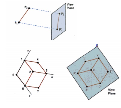
Parallel Projection:

Parallel projection is a method for generating a view of a solid object is to project points on the object surface along parallel lines onto the display plane.

In parallel projection, parallel lines in the world coordinate scene project into parallel lines on the two dimensional display planes.

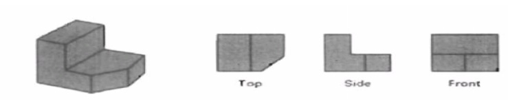
This technique is used in engineering and architectural drawings to represent an object with a set of views that maintain relative proportions of the object.

The appearance of the solid object can be reconstructed from the major views

Perspective Projection:

It is a method for generating a view of a three dimensional scene is to project points to the display plane alone converging paths.

This makes objects further from the viewing position be displayed smaller than objects of the same size that are nearer to the viewing position.

In a perspective projection, parallel lines in a scene that are not parallel to the display plane are projected into converging lines.

SIGNIFICANCE:

Scenes displayed using perspective projections appear more realistic, since this is the way that our eyes and a camera lens form images.

2. THREE-DIMENSIONAL OBJECT REPRESENTATIONS

CONCEPT

Three Dimensional Object Representations

Representation schemes for solid objects are divided into two categories as follows: 1. Boundary Representation ( B-reps)

It describes a three dimensional object as a set of surfaces that separate the object interior from the environment. Examples are polygon facets and spline patches.

2. Space Partitioning representation

Eg: Octree Representation

SIGNIFICANCE:

It Describes The Interior Properties, By Partitioning The Spatial Region Containing An Object Into A Set Of Small, Nonoverlapping, Contiguous Solids(Usually Cubes).

3. POLYGON SURFACES POLYGONTABLES- PLANE EQUATIONS - POLYGON MESHES

CONCEPT

Polygon surfaces are boundary representations for a 3D graphics object is a set of polygons that enclose the object interior. Polygon Tables

The polygon surface is specified with a set of vertex coordinates and associated attribute parameters.

For each polygon input, the data are placed into tables that are to be used in the subsequent processing.

Polygon data tables can be organized into two groups: Geometric tables and attribute tables.

Geometric Tables

Contain vertex coordinates and parameters to identify the spatial orientation of the polygon surfaces. Attribute tables Contain attribute information for an object such as parameters specifying the degree of transparency of the object and its surface reflectivity and texture characteristics.

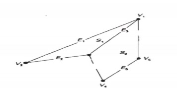
Vertex table Edge Table Polygon surface table V1 : X1, Y1, Z1 E1 : V1, V2 S1 : E1, E2, E3 V2 : X2, Y2, Z2 E2 : V2, V3 S2 : E3, E4, E5, E6 V3 : X3, Y3, Z3 E3 : V3, V1 V4 : X4, Y4, Z4 E4 : V3, V4 V5 : X5, Y5, Z5 E5 : V4, V5 E6 : V5, V1

Listing the geometric data in three tables provides a convenient reference to the individual components (vertices, edges and polygons) of each object.

The object can be displayed efficiently by using data from the edge table to draw the component lines.

Extra information can be added to the data tables for faster information extraction. For instance, edge table can be expanded to include forward points into the polygon table so that common edges between polygons can be identified more rapidly.

vertices are input, we can calculate edge slopes and we can scan the coordinate values to identify the minimum and maximum x, y and z values for individual polygons.

The more information included in the data tables will be easier to check for errors.

Some of the tests that could be performed by a graphics package are:

1.That every vertex is listed as an endpoint for at least two edges.

2.That every edge is part of at least one polygon.

3.That every polygon is closed.

4.That each polygon has at least one shared edge.

5.That if the edge table contains pointers to polygons, every edge referenced by a polygon pointer has a reciprocal pointer back to the polygon.

Plane Equations:

To produce a display of a 3D object, we must process the input data representation for the object through several procedures such as,

- Transformation of the modeling and world coordinate descriptions to viewing coordinates.

- Then to device coordinates:

- Identification of visible surfaces

- The application of surface-rendering procedures.

For these processes, we need information about the spatial orientation of the individual surface components of the object. This information is obtained from the vertex coordinate value and the equations that describe the polygon planes.

The equation for a plane surface is Ax + By+ Cz + D = 0 ----(1) Where (x, y, z) is any point on the plane, and the coefficients A,B,C and D are constants describing the spatial properties of the plane.

Polygon Meshes

A single plane surface can be specified with a function such as fillArea. But when object surfaces are to be tiled, it is more convenient to specify the surface facets with a mesh function.

One type of polygon mesh is the triangle strip.A triangle strip formed with 11 triangles connecting 13 vertices.

This function produces n-2 connected triangles given the coordinates for n vertices.

4. CURVED LINES AND SURFACES

CONCEPT:

Displays of three dimensional curved lines and surface can be generated from an input set of mathematical functions defining the objects or from a set of user specified data points.

When functions are specified, a package can project the defining equations for a curve to the display plane and plot pixel positions along the path of the projected function.

For surfaces, a functional description in decorated to produce a polygon-mesh approximation to the surface.

5. QUADRIC SURFACES

The quadric surfaces are described with second degree equations (quadratics).

They include spheres, ellipsoids, tori, parabolids, and hyperboloids.

Sphere

In Cartesian coordinates, a spherical surface with radius r centered on the coordinates origin is defined as the set of points (x, y, z) that satisfy the equation.

x2 + y2 + z2 = r2

Ellipsoid

Ellipsoid surface is an extension of a spherical surface where the radius in three mutually perpendicular directions can have different values

6. SPLINE REPRESENTATIONS

CONCEPT:

A Spline is a flexible strip used to produce a smooth curve through a designated set of points.

Several small weights are distributed along the length of the strip to hold it in position on the drafting table as the curve is drawn.

The Spline curve refers to any sections curve formed with polynomial sections satisfying specified continuity conditions at the boundary of the pieces.

A Spline surface can be described with two sets of orthogonal spline curves.

Splines are used in graphics applications to design curve and surface shapes, to digitize drawings for computer storage, and to specify animation paths for the objects or the camera in the scene. CAD applications for splines include the design of automobiles bodies, aircraft and spacecraft surfaces, and ship hulls.

Interpolation and Approximation Splines

Spline curve can be specified by a set of coordinate positions called control points which indicates the general shape of the curve.

These control points are fitted with piecewise continuous parametric polynomial functions in one of the two ways.

When polynomial sections are fitted so that the curve passes through each control point the resulting curve is said to interpolate the set of control points.

A set of six control points interpolated with piecewise continuous polynomial sections

When the polynomials are fitted to the general control point path without necessarily passing through any control points, the resulting curve is said to approximate the set of control points.

A set of six control points approximated with piecewise continuous polynomial sections

Interpolation curves are used to digitize drawings or to specify animation paths.

Approximation curves are used as design tools to structure object surfaces.

A spline curve is designed , modified and manipulated with operations on the control points.The curve can be translated, rotated or scaled with transformation applied to the control points.

The convex polygon boundary that encloses a set of control points is called the convex hull.

The shape of the convex hull is to imagine a rubber band stretched around the position of the control points so that each control point is either on the perimeter of the hull or inside it.

Parametric Continuity Conditions

For a smooth transition from one section of a piecewise parametric curve to the next various continuity conditions are needed at the connection points.

If each section of a spline in described with a set of parametric coordinate functions or the form

x = x(u), y = y(u), z = z(u), u1<= u <= u2

Zero order parametric continuity referred to as C0 continuity, means that the curves meet. (i.e) the values of x,y, and z evaluated at u2 for the first curve section are equal. Respectively, to the value of x,y, and z evaluated at u1 for the next curve section.

First order parametric continuity referred to as C1 continuity means that the first parametric derivatives of the coordinate functions in equation (a) for two successive curve sections are equal at their joining point.

Second order parametric continuity, or C2 continuity means that both the first and second parametric derivatives of the two curve sections are equal at their intersection.

Geometric Continuity Conditions

To specify conditions for geometric continuity is an alternate method for joining two successive curve sections.

The parametric derivatives of the two sections should be proportional to each other at their common boundary instead of equal to each other.

Zero order Geometric continuity referred as G0 continuity means that the two curves sections must have the same coordinate position at the boundary point.

First order Geometric Continuity referred as G1 continuity means that the parametric first derivatives are proportional at the interaction of two successive sections.

Second order Geometric continuity referred as G2 continuity means that both the first and second parametric derivatives of the two curve sections are proportional at their boundary. Here the curvatures of two sections will match at the joining position.

SIGNIFICANCE:

A spline curve is designed , modified and manipulated with operations on the control points.The curve can be translated, rotated or scaled with transformation applied to the control points.

7. VISUALIZATION OF DATA SETS

CONCEPT:

The use of graphical methods as an aid in scientific and engineering analysis is commonly referred to as scientific visualization.

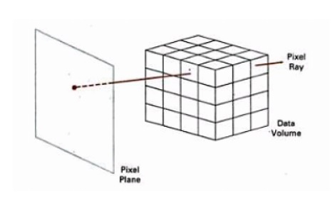
This involves the visualization of data sets and processes that may be difficult or impossible to analyze without graphical methods. Example medical scanners, satellite and spacecraft scanners.

Visualization techniques are useful for analyzing process that occur over a long period of time or that cannot observed directly. Example quantum mechanical phenomena and special relativity effects produced by objects traveling near the speed of light.

Scientific visualization is used to visually display , enhance and manipulate information to allow better understanding of the data.

Similar methods employed by commerce , industry and other nonscientific areas are sometimes referred to as business visualization.

Data sets are classified according to their spatial distribution ( 2D or 3D ) and according to data type (scalars , vectors , tensors and multivariate data ).

Visual representation for Vector fields

A vector quantity V in three-dimensional space has three scalar values ( Vx , Vy,Vz, ) one for each coordinate direction, and a two-dimensional vector has two components (Vx, Vy,). Another way to describe a vector quantity is by giving its magnitude IV I and its direction as a unit vector u. As with scalars, vector quantities may be functions of position, time, and other parameters. Some examples of physical vector quantities are velocity, acceleration, force, electric fields, magnetic fields, gravitational fields, and electric current.

One way to visualize a vector field is to plot each data point as a small arrow that shows the magnitude and direction of the vector. This method is most often used with cross-sectional slices, since it can be difficult to see the trends in a three-dimensional region cluttered with overlapping arrows. Magnitudes for the vector values can be shown by varying the lengths of the arrows. 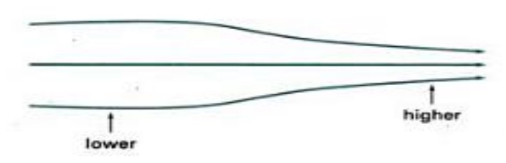Vector values are also represented by plotting field lines or streamlines . Field lines are commonly used for electric , magnetic and gravitational fields. The magnitude of the vector values is indicated by spacing between field lines, and the direction is the tangent to the field.

Visual Representations for Tensor Fields

A tensor quantity in three-dimensional space has nine components and can be represented with a 3 by 3 matrix. This representation is used for a second-order tensor, and higher-order tensors do occur in some applications. Some examples of physical, second-order tensors are stress and strain in a material subjected to external forces, conductivity of an electrical conductor, and the metric tensor, which gives the properties of a particular coordinate space.

SIGNIFICANCE:

The use of graphical methods as an aid in scientific and engineering analysis is commonly referred to as scientific visualization.

7. THREE DIMENSIONAL GEOMETRIC AND MODELING TRANSFORMATIONS:

CONCEPT:

Geometric transformations and object modeling in three dimensions are extended from two-dimensional methods by including considerations for the z-coordinate

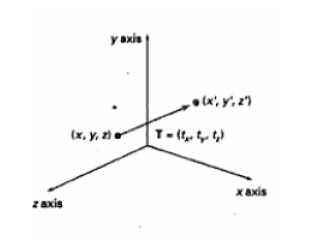
Translation

In a three dimensional homogeneous coordinate representation, a point or an object is translated from position P = (x,y,z) to position P’ = (x’,y’,z’) with the matrix operation.

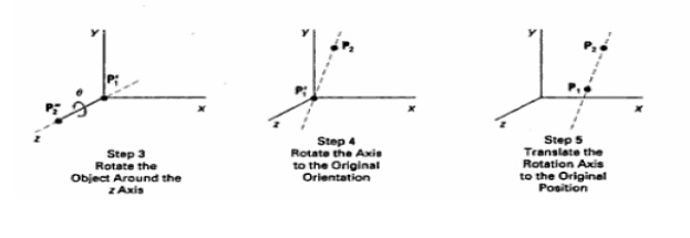
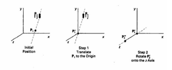
Rotation

To generate a rotation transformation for an object an axis of rotation must be designed to rotate the object and the amount of angular rotation is also be specified.

Positive rotation angles produce counter clockwise rotations about a coordinate axis.

Co-ordinate Axes Rotations

The 2D z axis rotation equations are easily extended to 3D. x = x cos θ – y sin θ

Scaling

The matrix expression for the scaling transformation of a position P = (x,y,.z)

Scaling an object changes the size of the object and repositions the object relatives to the coordinate origin.

If the transformation parameters are not equal, relative dimensions in the object are changed. The original shape of the object is preserved with a uniform scaling (sx = sy= sz) .

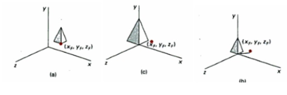
Scaling with respect to a selected fixed position (x f, yf, zf) can be represented with the following transformation sequence:

1.     Translate the fixed point to the origin. 2. Scale the object relative to the coordinate origin

Other Transformations

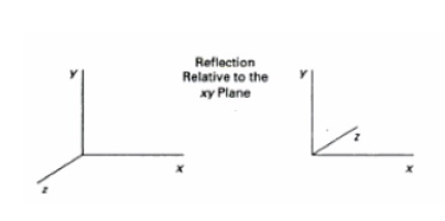
Reflections

A 3D reflection can be performed relative to a selected reflection axis or with respect to a selected reflection plane.

Reflection relative to a given axis are equivalent to 1800 rotations about the axis. Reflection relative to a plane are equivalent to 1800 rotations in 4D space.

When the reflection plane in a coordinate plane ( either xy, xz or yz) then the transformation can be a conversion between left-handed and right-handed systems.

Shears

Shearing transformations are used to modify object shapes.

They are also used in three dimensional viewing for obtaining general projections transformations.

The following transformation produces a z-axis shear.

Composite Transformation

Composite three dimensional transformations can be formed by multiplying the matrix representation for the individual operations in the transformation sequence.

This concatenation is carried out from right to left, where the right most matrixes is the first transformation to be applied to an object and the left most matrix is the last transformation.

A sequence of basic, three-dimensional geometric transformations is combined to produce a single composite transformation which can be applied to the coordinate definition of an object.

Three Dimensional Transformation Functions

Some of the basic 3D transformation functions are: translate ( translateVector, matrixTranslate) rotateX(thetaX, xMatrixRotate) rotateY(thetaY, yMatrixRotate) rotateZ(thetaZ, zMatrixRotate) scale3 (scaleVector, matrixScale)

Each of these functions produces a 4 by 4 transformation matrix that can be used to transform coordinate positions expressed as homogeneous column vectors.

Parameter translate Vector is a pointer to list of translation distances tx, ty, and tz.

Parameter scale vector specifies the three scaling parameters sx, sy and sz.

Rotate and scale matrices transform objects with respect to the coordinate origin.

Composite transformation can be constructed with the following functions:

composeMatrix3 buildTransformationMatrix3 composeTransformationMatrix3 The order of the transformation sequence for the buildTransformationMarix3 and composeTransfomationMarix3 functions, is the same as in 2 dimensions:

1.scale

2.rotate

3.translate

Once a transformation matrix is specified, the matrix can be applied to specified points with

transformPoint3 (inPoint, matrix, outpoint)

The transformations for hierarchical construction can be set using structures with the function

setLocalTransformation3 (matrix, type) where parameter matrix specifies the elements of a 4 by 4 transformation matrix and parameter type can be assigned one of the values of: Preconcatenate, Postconcatenate, or replace.

SIGNIFICANCE:

A 3D reflection can be performed relative to a selected reflection axis or with respect to a selected reflection plane.

8. THREE-DIMENSIONAL VIEWING

CONCEPT:

In three dimensional graphics applications,

- we can view an object from any spatial position, from the front, from above or from the back.

-  We could generate a view of what we could see if we were standing in the middle of a group of objects or inside object, such as a building.

Viewing Pipeline:

In the view of a three dimensional scene, to take a snapshot we need to do the following steps.

1.Positioning the camera at a particular point in space.

2.Deciding the camera orientation (i.e.,) pointing the camera and rotating it around the line of right to set up the direction for the picture.

3.When snap the shutter, the scene is cropped to the size of the „window  of the camera and light from the visible surfaces is projected into the camera film.

In such a way the below figure shows the three dimensional transformation pipeline, from modeling coordinates to final device coordinate.

Processing Steps

1.     Once the scene has been modeled, world coordinates position is converted to viewing coordinates.

2.The viewing coordinates system is used in graphics packages as a reference for specifying the observer viewing position and the position of the projection plane.

3.  Projection operations are performed to convert the viewing coordinate description of the scene to coordinate positions on the projection plane, which will then be mapped to the output device.

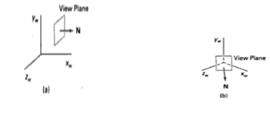
A viewplane or projection plane is set-up perpendicular to the viewing Zv axis.

World coordinate positions in the scene are transformed to viewing coordinates, then viewing coordinates are projected to the view plane.

The view reference point is a world coordinate position, which is the origin of the viewing coordinate system. It is chosen to be close to or on the surface of some object in a scene.

2.     Then we select the positive direction for the viewing Zv axis, and the orientation of the view plane by specifying the view plane normal vector, N. Here the world coordinate position establishes the direction for N relative either to the world origin or to the viewing coordinate origin.

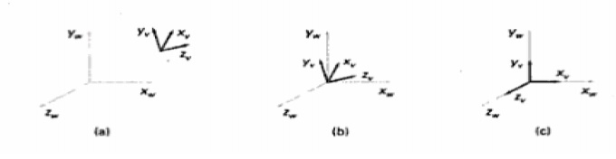
Transformation from world to viewing coordinates

Before object descriptions can be projected to the view plane, they must be transferred to viewing coordinate. This transformation sequence is,

1.Translate the view reference point to the origin of the world coordinate system.

2.Apply rotations to align the xv, yv and zv axes with the world xw,yw and zw axes respectively.

If the view reference point is specified at world position(x0,y0,z0) this point is translated to the world origin with the matrix transformation.

Another method for generation the rotation transformation matrix is to calculate unit uvn vectors and form the composite rotation matrix directly.

Given vectors N and V, these unit vectors are calculated as

n = N / (|N|) = (n1, n2, n3) u = (V*N) / (|V*N|) = (u1, u2, u3) v = n*u = (v1, v2, v3) This method automatically adjusts the direction for v, so that v is perpendicular to n.

The composite rotation matrix for the viewing transformation is

u1 u2 u3 0 R = v1 v2 v3 0 n1 n2 n3 0 0 0 0 1

which transforms u into the world xw axis, v onto the yw axis and n onto the zw axis

Projections

Once world coordinate descriptions of the objects are converted to viewing coordinates, we can project the 3 dimensional objects onto the two dimensional view planes.

There are two basic types of projection.

1. Parallel Projection - Here the coordinate positions are transformed to the view plane along parallel lines.

Parallel projection of an object to the view plan

SIGNIFICANCE:

In three dimensional graphics applications, we can view an object from any spatial position, from the front, from above or from the back.

9. VISIBLE SURFACE IDENTIFICATION

CONCEPT

A major consideration in the generation of realistic graphics displays is identifying those parts of a scene that are visible from a chosen viewing position.

Classification of Visible Surface Detection Algorithms

These are classified into two types based on whether they deal with object definitions directly or with their projected images

1. Object Space Methods:

compares objects and parts of objects to each other within the scene definition to determine which surfaces as a whole we should label as visible.

2. Image space methods:

visibility is decided point by point at each pixel position on the projection plane. Most Visible Surface Detection Algorithms use image space methods.

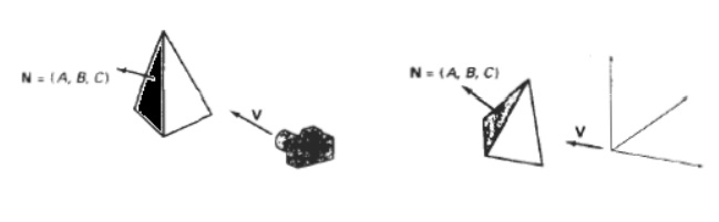
Back Face Detection

A point (x, y,z) is "inside" a polygon surface with plane parameters A, B, C, and D if Ax + By + Cz + D < 0 ----------------(1 ) When an inside point is along the line of sight to the surface, the polygon must be a back face .

Depth Buffer Method

A commonly used image-space approach to detecting visible surfaces is the depth-buffer method, which compares surface depths at each pixel position on the projection plane.

This procedure is also referred to as the z-buffer method. Each surface of a scene is processed separately, one point at a time across the surface. The method is usually applied to scenes containing only polygon surfaces, because depth values can be computed very quickly and the method is easy to implement.

But the mcthod can be applied to nonplanar surfaces. With object descriptions converted to projection coordinates, each (x, y, z) position on a polygon surface corresponds to the orthographic projection point (x, y) on the view plane.

We can implement the depth-buffer algorithm in normalized coordinates, so that z values range from 0 at the back clipping plane to Zmax at the front clipping plane.

Two buffer areas are required.A depth buffer is used to store depth values for each (x, y) position as surfaces are processed, and the refresh buffer stores the intensity values for each position.

Initially,all positions in the depth buffer are set to 0 (minimum depth), and the refresh buffer is initialized to the background intensity. We summarize the steps of a depth-buffer algorithm as follows: 1. Initialize the depth buffer and refresh buffer so that for all buffer positions (x, y), depth (x, y)=0, refresh(x , y )=Ibackgnd 2. For each position on each polygon surface, compare depth values to previously stored values in the depth buffer to determine visibility.

Calculate the depth z for each (x, y) position on the polygon.

If z > depth(x, y), then set

depth ( x, y)=z , refresh(x,y)= Isurf(x, y)

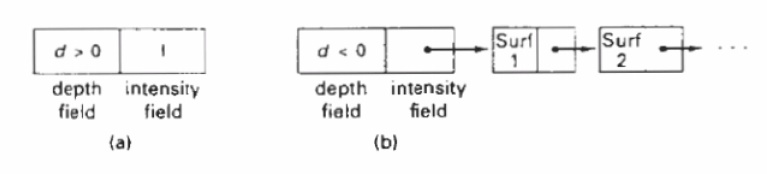
A- BUFFER METHOD

An extension of the ideas in the depth-buffer method is the A-buffer method. The A buffer method represents an antialiased, area-averaged, accumulation-buffer method developed by Lucasfilm for implementation in the surface-rendering system called REYES (an acronym for "Renders

Everything You Ever Saw"). A drawback of the depth-buffer method is that it can only find one visible surface at each pixel position. The A-buffer method expands

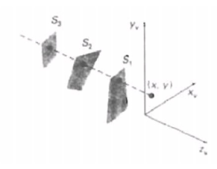
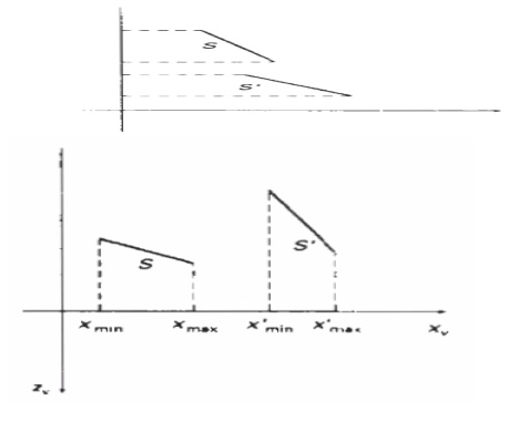
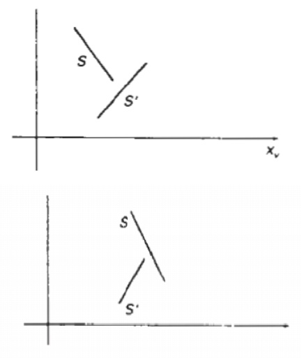
SCAN-LINE METHOD

This image-space method for removing hidden surfaces is an extension of the scan-line algorithm for filling polygon interiors. As each scan line is processed, all polygon surfaces intersecting that line are examined to determine which are visible. Across each scan line, depth calculations are made for each overlapping surface to determine which is nearest to the view plane. When the visible surface has been determined, the intensity value for that position is entered into the refresh buffer.

We assume that tables are set up for the various surfaces, which include both an edge table and a polygon table. The edge table contains coordinate endpoints for each line in-the scene, the inverse slope of each line, and pointers into the polygon table to identify the surfaces bounded by each line. The polygon table contains coefficients of the plane equation for each surface, intensity information for the surfaces, and possibly pointers into the edge table.

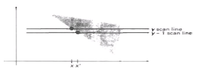
To facilitate the search for surfaces crossing a given scan line, we can set up an active list of edges from information in the edge table. This active list will contain only edges that cross the current scan line, sorted in order of increasing x. In addition, we define a flag for each surface that is set on or off to indicate whether a position along a scan line is inside or outside of the surface. Scan lines are processed from left to right. At the leftmost boundary of a surface, the surface flag is turned on; and at the rightmost boundary, it is turned off.

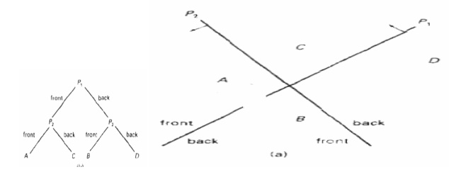
BSP-Tree Method A binary space-partitioning (BSP) tree is an efficient method for determining object visibility by painting surfaces onto the screen from back to front, as in the painter's algorithm. The BSP tree is particularly useful when the view reference point changes, but the objects in a scene are at fixed positions. Applying a BSP tree to visibility testing involves identifying surfaces that are "inside" and "outside" the partitioning plane at each step of the space subdivision, relative to the viewing direction. The figure(a) illustrates the basic concept in this algorithm.

Area – Subdivision Method

This technique for hidden-surface removal is essentially an image-space method ,but object-space operations can be used to accomplish depth ordering of surfaces. The area-subdivision method takes advantage of area coherence in a scene by locating those view areas that represent part of a single surface. We apply this method by successively dividing the total viewing area into smaller and smaller rectangles until each small area is the projection of part of a single visible surface or no surface at all.

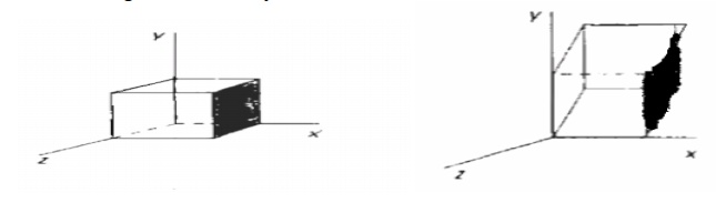
octree methods

When an octree representation is used for the viewing volume, hidden-surface elimination is accomplished by projecting octree nodes onto the viewing surface in a front-to-back order. In the below Fig. the front face of a region of space (the side toward the viewer) is formed with octants 0, 1, 2, and 3. Surfaces in the front of these octants are visible to the viewer. Any surfaces toward the re in the back octants (4,5,6, and 7) may be hidden by the front surfaces.

When an octree representation is used for the viewing volume, hidden-surface elimination is accomplished by projecting octree nodes onto the viewing surface in a front-to-back order. In the below Fig. the front face of a region of space (the side toward the viewer) is formed with octants 0, 1, 2, and 3. Surfaces in the front of these octants are visible to the viewer. Any surfaces toward the re in the back octants (4,5,6, and 7) may be hidden by the front surfaces.

SIGNIFICANCE:

This technique for hidden-surface removal is essentially an image-space method ,but object-space operations can be used to accomplish depth ordering of surfaces.

APPLICATIONS:

1.Real time 3D magic

2.Implement 3D transformations

3.Correct view about 3D