Traverse (surveying) and Types Of Traverse

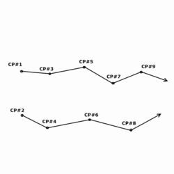
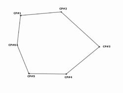
Diagram of a closed traverse

Open/Free

An open, or free traverse (link traverse) consist of known points plotted in any corresponding linear direction, but do not return to the starting point or close upon a point of equal or greater order accuracy. It allows geodetic triangulation for sub-closure of three known points; known as the "Bowditch rule" or "compass rule" in geodetic science and surveying, which is the principle that the linear error is proportional to the length of the side in relation to the perimeter of the traverse

•         Open survey is utilised in plotting a strip of land which can then be used to plan a route in road construction. The terminal (ending) point is always listed as unknown from the observation point.

Closed

A closed traverse (polygonal, or loop traverse) is a practice of traversing when the terminal point closes at the starting point. The control points may envelop, or are set within the boundaries, of the control network. It allows geodetic triangulation for sub-closure of all known observed points.

•         Closed traverse is useful in marking the boundaries of wood or lakes. Construction and civil engineers utilize this practice for preliminary surveys of proposed projects in a particular designated area. The terminal (ending) point closes at the starting point.

•         Control point - the primary/base control used for preliminary measurements; it may consist of any known point capable of establishing accurate control of distance and direction (i.e. coordinates, elevation, bearings, etc).

1.    Starting -It is the initial starting control point of the traverse.

2.     Observation -All known control points that are setted or observed within the traverse.

3.             Terminal -It is the initial ending control point of the traverse; its coordinates are unknown

Earthwork Computations

Computing earthwork volumes is a necessary activity for nearly all construction projects and is often accomplished as a part of route surveying, especially for roads and highways. Suppose, for example, that a volume of cut must be removed between two adjacent stations along a highway route. If the area of the cross section at each station is known, you can compute the average-end area (the average of the two cross-sectional areas) and then multiply that average end area by the known horizontal distance between the stations to determine the volume of cut.

To determine the area of a cross section easily, you can run a planimeter around the plotted outline of the section. Counting the squares, explained in chapter 7 of this traman, is another way to determine the area of a cross section. Three other methods are explained below.

AREA BY RESOLUTION.- Any regular or irregular polygon can be resolved into easily calculable geometric figures, such as triangles andABH and DFE, and two trapezoids, BCGH and CGFD. For each of these figures, the approximate dimensions have been determined by the scale of the plot. From your knowledge of mathematics, you know that the area of each triangle can be determined using the following formula:

A [s(s-a)(s-b)(s-c)]^1/2

s = one half of the perimeter of the triangle,

and that for each trapezoid, you can calculate the area using the formula: Where:

A = ½(b₁+b₂)h

When the above formulas are applied and the sum of the results are determined, you find that the total area of the cross section at station 305 is 509.9 square feet.

AREA BY FORMULA.- A regular section area for a three-level section can be more exactly determined by applying the following formula:

Figure 10-4.-A cross section plotted on cross-section paper.

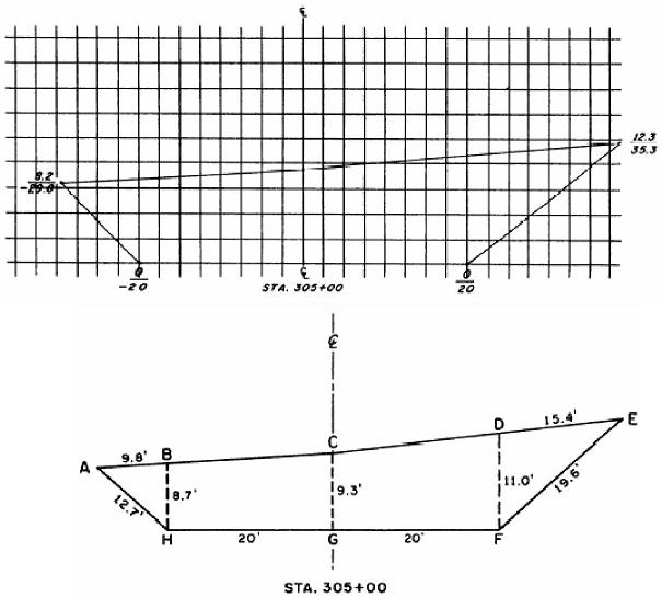
Figure10-6 forirregularsections

determine the area of sections of this kind, you should use a method of determining area by coordinates. For explanation purpose, let'sconsider station 305 (fig. 10-6). First, consider the point where the center line intersects the grade line as the point of origin for the coordinates. Vertical distances above the grade line are positive Y coordinates; vertical distances below the grade line are negative Y coordinates. A point on the grade line itself has a Y coordinate of 0. Similarly, horizontal distances to the right of the center line are positive X coordinates; distances to the left of the center line are negative X coordinates; and any point on the center line itself has an X coordinate of 0.

Plot the cross section, as shown in figure 10-7, and be sure that the X and Y coordinates have their proper signs. Then, starting at a particular point and going successively in a clockwise direction, write down the coordinates, as shown in figure 10-8.

After writing down the coordinates, you then multiply each upper term by the algebraic difference of the following lower term and the preceding lower term, as indicated by the direction of the arrows (fig. 10-8). The algebraic sum of the resulting products is the double area of the cross section. Proceed with the computation as follows:

Figure 10-5.-Cross section resolved into triangles and trapezoids.

A=w/4 . (h₁+h₂)    +   C/2.(d₁+d₂)

the formula for station 305 + 00 (fig. 10-4), you get the following results:

A = (40/4)(8.2+ 12.3)+ (9.3/2)(29.8+ 35.3)= 507.71 square feet.

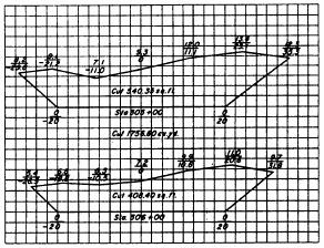
AREA OF FIVE-LEVEL OR IRREGULAR SECTION.- Figures 10-6 and 10-7 are the field notes and plotted cross sections for two irregular sections. To

Figure 10-6.-Field notes for irregular sections.

determine the area of sections of this kind, you should use a method of determining area by coordinates. For explanation purpose, let'sconsider station 305 (fig. 10-6). First, consider the point where the center line intersects the grade line as the point of origin for the coordinates. Vertical distances above the grade line are positive Y coordinates; vertical distances below the grade line are negative Y coordinates. A point on the grade line itself has a Y coordinate of 0. Similarly, horizontal distances to the right of the center line are positive X coordinates; distances to the left of the center line are negative X coordinates; and any point on the center line itself has an X coordinate of 0.

Plot the cross section, as shown in figure 10-7, and be sure that the X and Y coordinates have their proper signs. Then, starting at a particular point and going successively in a clockwise direction, write down the coordinates, as shown in figure 10-8.

After writing down the coordinates, you then multiply each upper term by the algebraic difference of the following lower term and the preceding lower term, as indicated by the direction of the arrows (fig. 10-8). The algebraic sum of the resulting products is the double area of the cross section. Proceed with the computation as follows:

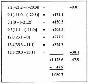
Since the result (1,080.70 square feet) represents the double area, the area of the cross section is one half of that amount, or 540.35 square feet. By similar method, the area of the cross section at station 306 (fig. 10-7) is 408.40 square feet.

EARTHWORK VOLUME.- As discussed previously, when you know the area of two cross sections, you can multiply the average of those cross-sectional areas by the known distance between them to obtain the volume of earth to be cut or filled. Consider figure 10-9 that shows the plotted cross sections of two sidehill sections. For this figure, when you multiply the average-end area (in fill) and the average-end area (in cut) by the distance between the two stations (100 feet), you obtain the estimated amount of cut and fill between the stations. In this case, the amount of space that requires filling is computed to be approximately 497.00 cubic yards and the amount of cut is about 77.40 cubic yards.

MASS DIAGRAMS.- A concern of the highway designer is economy on earthwork. He wants to know exactly where, how far, and how much earth to move in a section of road. The ideal situation is to balance the cut and fill and limit the haul distance. A technique for balancing cut and fill and determining the

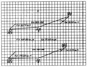
Figure 10-9.-Plots of two sidehill sections.

Figure 10-8.-Coordinates for cross-section station 305 shown in figure 10-7. economical haul distance is the mass diagram method.

A mass diagram is a graph or curve on which the algebraic sums of cuts and fills are plotted against linear distance. Before these cuts and fills are tabulated, the swells and compaction factors are considered in computing the yardage. Earthwork that is in place will yield more yardage when excavated and less yardage when being compacted. An example of this is sand: 100 cubic yards in place yields 111 cubic yards loose and only 95 cubic yards when compacted. Table 10-1 lists conversion factors for various types of soils. These factors should be used when you are preparing a table of cumulative yardage for a mass diagram. Cuts are indicated by a rise in the curve and are considered positive; fills are indicated by a drop in the curve and are considered negative. The yardage between any pair of stations can be determined by inspection. This feature makes the mass diagram a great help in the attempt to balance cuts and fills within the limits of economic haul.

The limit of economic haul is reached when the cost of haul and the cost of excavation become equal. Beyond that point it is cheaper to waste the cut from one place and to fill the adjacent hollow with material taken from a nearby borrow pit. The limit of economic haul will, of course, vary at different stations on the project, depending on the nature of the terrain, the availability of equipment, the type of material, accessibility, availability of manpower, and other considerations.