Chapter: Operations Research: An Introduction : Integer Linear Programming
Traveling Salesperson Problem (TSP)
TRAVELING SALESPERSON (TSP) PROBLEM
Historically, the TSP problem deals with finding the shortest (closed) tour in an n-city situation where each city is visited exactly once. The problem, in essence, is an assignment model that excludes subtours. Specifically, in an n-city situation, define
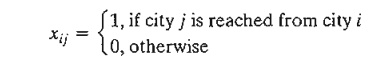
Given that dij is the distance from city i to city j, the TSP model is given as
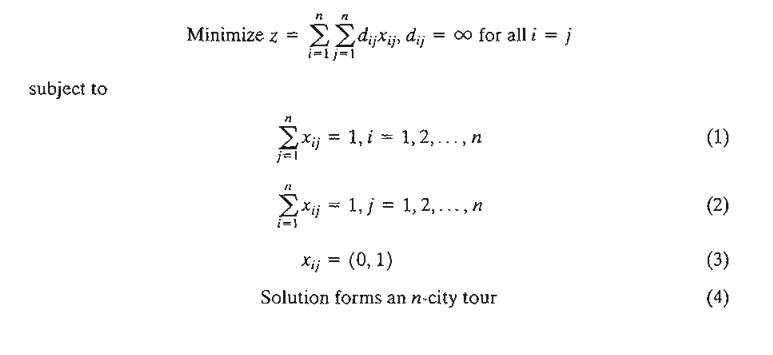
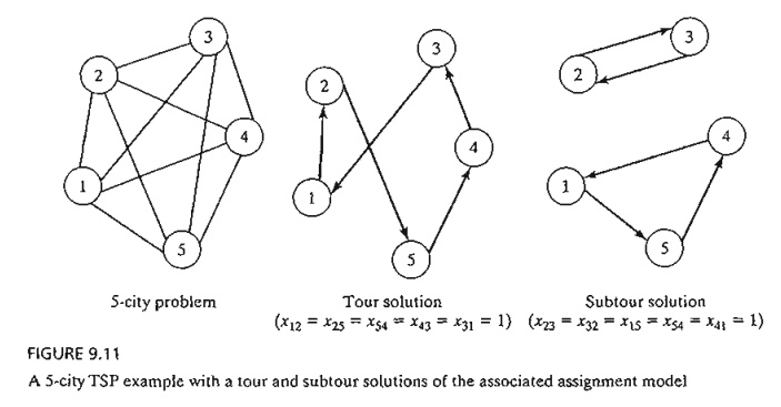
Constraints (1), (2), and (3) define a regular assignment model (Section 5.4). Figure 9.11 demonstrates a 5-city problem. The arcs represent two-way routes. The figure also illustrates a tour and a subtour solution of the associated assignment model. If the optimum solution of the assignment model (i.e., excluding constraint 4) happens to produce a tour, then it is also optimum for the TSP. Otherwise, restriction (4) must be accounted for to ensure a tour solution.
Exact solutions of the TSP problem include branch-and-bound and cutting-plane algorithms. Both are rooted in the ideas of the general B&B and cutting plane algo-rithms presented in Section 9.2. Nevertheless, the problem is typically difficult computationally, in the sense that either the size or the computational time needed to obtain a solution may become inordinately large. For this reason, heuristics are sometimes used to provide a "good" solution for the problem.
Before presenting the heuristic and exact solution algorithms, we present an ex-ample that demonstrates the versatility of the TSP model in representing other practi-cal situations (see also Problem Set 9.3a).
Example 9.3-1
The daily production schedule at the Rainbow Company includes batches of white (W), yellow (Y), red (R), and black (B) paints. Because Rainbow uses the same facilities for all four types of paint, proper cleaning between batches is necessary. The table below summarizes the clean-up time in minutes. Because each color is produced in a single batch, diagonal entries in the table are assigned infinite setup time. The objective is to determine the optimal sequencing for the daily production of the four colors that will minimize the associated total clean-up time.
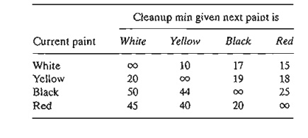
Each paint is thought of as a "city" and the "distances" are represented by the clean-up time needed to switch from one paint batch to the next. The situation reduces to determining the shortest loop that starts with one paint batch and passes through each of the remaining three paint batches exactly once before returning back to the starting paint.
We can solve this problem by exhaustively enumerating the six [(4 - 1)! = 3! = 6] possible loops of the network. The following table shows that W -> Y -> R -> B -> W is the optimum loop.
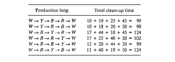
Exhaustive enumeration of the loops is not practical in general. Even a modest size 11-city problem will require enumerating 10! = 3,628,800 tours, a daunting task indeed. For this reason, the problem must be formulated and solved in a different manner, as we will show later in this section.
To develop the assignment-based formulation for the paint problem, define
Xij = 1 if paint j follows paint i and zero otherwise
Letting M be a sufficiently large positive value, we can formulate the Rainbow problem as
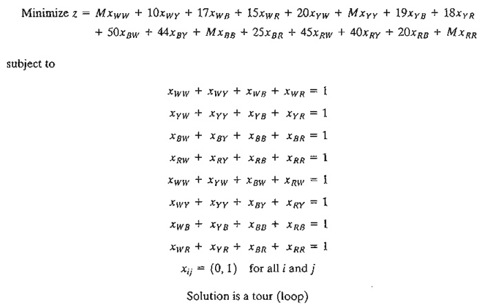
The use of M in the objective function guarantees that a paint job cannot follow itself. The same result can be realized by deleting Xww, XYY, XBB, and XRR from the entire model.
PROBLEM SET 9.3A
*1. A manager has a total of 10 employees working on six projects. There are overlaps among the assignments as the following table shows:
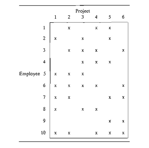
The manager meets with each employee individually once a week for a progress report. Each meeting lasts about 20 minutes for a total of 3 hours and 20 minutes for all 10 employees. To reduce the total time, the manager wants to hold group meetings depend-ing on shared projects. The objective is to schedule the meetings in a way that will reduce the traffic (number of employees) in and out of the meeting foam. Formulate the problem as a mathematical model.
2. A book salesperson who lives in Basin must call once a month on four customers located in Wald, Bon, Mena, and Kiln. The following table gives the distances in miles among the different cities.
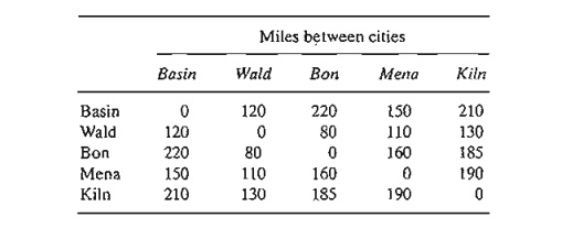
The objective is to minimize the total distance traveled by the salesperson. Formulate the problem as an assignment-based ILP.
3. Circuit boards (such as those used with PCs) are fitted with holes for mounting different electronic components. The holes are drilled with a movable drill. The following table pro-vides the distances (in centimeters) between pairs of 6 holes of a specific circuit board.
Formulate the assignment portion of an ILP representing this problem.
1. Heuristic Algorithms
This section presents two heuristics: the nearest-neighbor and the subtour-reversal algorithms. The first is easy to implement and the second requires more computations. The tradeoff is that the second algorithm generally yields better results. Ultimately, the two heuristics are combined into one heuristic, in which the output of the nearest-neighbor algorithm is used as input to the reversal algorithm.
The Nearest-Neighbor Heuristic. As the name of the heuristic suggests, a "good" solution of the TSP problem can be found by starting with any city (node) and then connecting it with the closest one. The just-added city is then linked to its nearest unlinked city (with ties broken arbitrarily). The process continues until a tour is formed.
Example 9.3-2
The matrix below summarizes the distances in miles in as-city TSP problem.
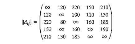
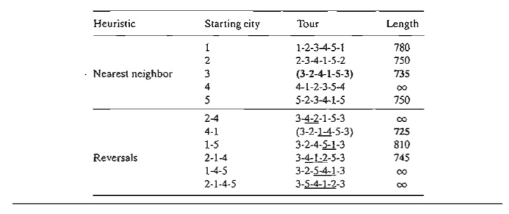
The heuristic can start from any of the five cities. Each starting city may lead to a different tour. The following table provides the steps of the heuristic starting at city 3.
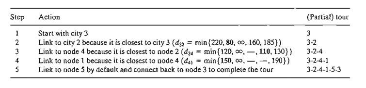
Notice the progression of the steps: Comparisons exclude distances to nodes that are part of a constructed partial tour. These are indicated by (-) in the Action column of the table.
The resulting tour 3-2-4-1-5-3 has a total length of 80 + 110 + 150 + 210 + 185 = 735 miles. Observe that the quality of the heuristic solution is starting-node dependent. For example, starting from node 1, the constructed tour is 1-2-3-4-5-1 with a total length of 780 miles (try it!).
Subtour Reversal Heuristic. In an n-city situation, the subtour reversal heuristic starts with a feasible tour and then tries to improve on it by reversing 2-city subtours, followed by 3-city subtours, and continuing until reaching subtours of size n - 1.
Example 9.3-3
Consider the problem of Example 9.3-2. The reversal steps are carried out in the following table using the feasible tour 1-4-3-5-2-1 of length 745 miles:
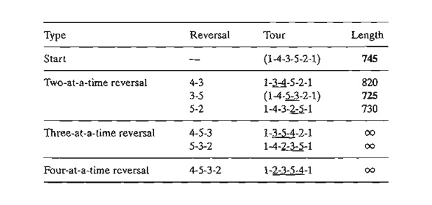
The two-at-a-time reversals of the initial tour 1-4-3-5-2-1 are 4-3, 3-5, and 5-2, which leads to the given tours with their associated lengths of 820, 725, and 730. Since 1-4-5-3-2-1 yields a smaller length (= 725), it is used as the starting tour for making the three-at-a-time reversals. As shown in the table, these reversals produce no better results. The same result applies to the four-at-a-time reversal. Thus, 1-4-5-3-2-1 (with length 725 miles) provides the best solution of heuristic.
Notice that the three-at-a-time reversals did not produce a better tour, and, for this rea-son, we continued to use the best two-at-a-time tour with the four-at-a-time reversal. Notice also that the reversals do not include the starting city of the tour (= 1 in this example) because the process does not yield a tour. For example, the reversal 1-4 leads to 4-1-3-5-2-1, which is not a tour.
The solution determined by the reversal heuristic is a function of the initial feasible tour used to start the algorithm. For example, if we start with 2-3-4-1-5-2 with length 750 miles, the heuristic produces the tour 2-1-4-3-5-2 with length 745 miles (verify!), which is inferior to the solution we have in the table above. For this reason, it may be advantageous to first utilize the nearest-neighbor heuristic to determine all the tours that result from using each city as a starting node and then select the best as the starting tour for the reversal heuristic. This combined heuristic should, in general, lead to superior solutions than if either heuristic is applied separately. The following table shows the application of the composite heuristic to the present example.
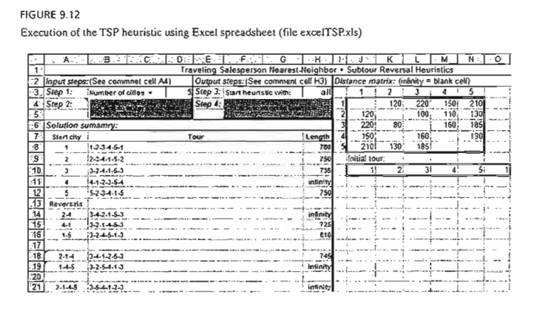
Excel Moment.
Figure 9.12 provides a general Excel template (file exceITSP.xls) for the heuristics. It uses three execution options depending on the entry in cell H3:
1. If you enter a city number, the nearest-neighbor heuristic is used to find a tour starting with the designated city.
2. If you enter the word "tour" (without the quotes), you must simultaneously provide an initial feasible tour in the designated space. In this case, only the reversal heuristic is applied to the tour you provided.
3. If you enter the word "all," the nearest-neighbor heuristic is used first, and its best tour is then used to execute the reversal heuristic.
File exceITSP.v2.xls automates the operations of Step 3.
2. B&B Solution Algorithm
The idea of the B&B algorithm is to start with the optimum solution of the associated assignment problem. If the solution is a tour, the process ends. Otherwise, restrictions are imposed to remove the subtours. This can be achieved by creating as many branch-es as the number of xij variables associated with one of the subtours. Each branch will correspond to setting one of the variables of the subtour equal to zero (recall that all the variables associated with a subtour equal 1). The solution of the resulting assign-ment problem mayor may not produce a tour. If it does, we use its objective value as an upper bound on the true minimum tour length. If it does not, further branching is necessary, again creating as many branches as the number of variables in one of the subtours. The process continues until all unexplored subproblems have been fathomed, either by producing a better (smaller) upper bound or because there is evidence that the subproblem cannot produce a better solution. The optimum tour is the one associ-ated with the best upper bound.
The following example provides the details of the TSP B&B algorithm.
Example 9.3-4
Consider the following 5-city TSP problem:
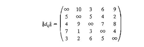
We start by solving the associated assignment, which yields the following solution:
z = 15, (x13 = x31 = 1), (x25 = x54 = x42 = 1), all others = 0
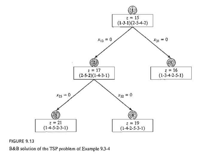
This solution yields two subtours: (1-3-1) and (2-5-4-2), as shown at node 1 in Figure 9.13. The associated total distance is z = 15, which provides a lower bound on the optimal length of the 5-city tour.
A straightforward way to determine an upper bound is to select any tour and use its length as an upper bound estimate. For example, the tour 1-2-3-4-5-1 (selected totally arbitrarily) has a total length of 10 + 5 + 7 + 4 + 3 = 29. Alternatively, a better upper bound can be found by applying the heuristic of Section 9.3.1. For the moment, we will use the upper bound of length 29 to apply the B&B algorithm. Later, we use the "improved" upper bound obtained by the heuristic to demonstrate its impact on the search tree.
The computed lower and upper bounds indicate that the optimum tour length lies in range (15, 29). A solution that yields a tour length larger than (or equal to) 29 is discarded as nonpromising.
To eliminate the subtours at node 1, we need to "disrupt" its loop by forcing its member variables, xij, to be zero. Subtour 1-3-1 is disrupted if we impose the restriction xl3 = 0 or x31 = 0 (i.e., one at a time) on the assignment problem at node 1. Similarly, subtour 2-5-4-2 is eliminated by imposing one of the restrictions x25 = 0, x54 = 0, or x42 = 0. In terms of the B&B tree, each of these restrictions gives rise to a branch and hence a new subproblem. It is important to notice that branching both subtours at node 1 is not necessary. Instead, only one subtour needs to be disrupted at anyone node. The idea is that a breakup of one subtour automatically alters the member variables of the other subtour and hence produces conditions that are favorable to creating a tour. Under this argument, it is more efficient to select the subtour with the smallest number of cities because it creates the smallest number of branches.
Targeting subtour (1-3-1), two branches x13 = 0 and x31 = 0 are created at node 1. The associated assignment problems are constructed by removing the row and column associated with the zero variable, which makes the assignment problem smaller. Another way to achieve the same result is to leave the size of the assignment problem unchanged and simply assign an infinite distance to the branching variable. For example, the assignment problem associated with xl3 = 0 requires substituting d13 = ¥ in the assignment model at node 1. Similarly, for x31 = 0, we substitute d31 = ¥.
In Figure 9.13, we arbitrarily start by solving the subproblem associated with x13 = 0 by setting dl3 = ¥, Node 2 gives the solution z = 17 but continues to produce the subtours (2-5-2) and (1-4-3-1). Repeating the procedure we applied at node 1 gives rise to two branches: x25 = 0 and x52 = 0.
We now have three unexplored subproblems, one from node 1 and two from node 2, and we are free to investigate any of them at this point. Arbitrarily exploring the subproblem associated with x25 = 0 from node 2, we set d13 = ¥ and d25 = ¥ in the original assignment problem, which yields the solution z = 21 and the tour solution 1-4-5-2-3-1 at node 3. The tour solution at node 3 lowers the upper bound from z == 29 to z == 21. This means that any unexplored subproblem that can be shown to yield a tour length larger than 21 is discarded as nonpromising.
We now have two unexplored subproblems. Selecting the subproblem 4 for exploration, we set dl3 = ¥ and d52 = ¥ in the original assignment, which yields the tour solution 1-4-2-5-3-1 with z = 19. The new solution provides a better tour than the one associated with the current upper bound of 21. Thus, the new upper bound is updated to z = 19 and its associated tour, 1-4-2-5-3-1, is the best available so far.
Only subproblem 5 remains unexplored. Substituting d31 = ¥ in the original assignment problem at node 1, we get the tour solution 1-3-4-2-5-1 with z = 16, at node 5. Once again, this is a better solution than the one associated with node 4 and thus requires updating the upper bound to z = 16.
There are no remaining unfathomed nodes, which completes the search tree. The optimal tour is the one associated with the current upper bound: 1-3-4-2-5-1 with length 16 miles.
Remarks. The solution of the example reveals two points:
1. Although the search sequence 1 -> 2 -> 3 -> 4 -> 5 was selected deliberately to demonstrate the mechanics of the B&B algorithm and the updating of its upper bound, we generally have no way of predicting which sequence should be adopted to improve the efficiency of the search. Some rules of thumb can be of help. For example, at a given node we can start with the branch associated with the largest dij among all the created branches. By canceling the tour leg with the largest dij, the hope is that a "good" tour with a smaller total length will be found. In the present example, this rule calls for exploring branch x31 == 0 to node 5 be-fore branch x13 to node 2 because (d31 == 4) > (d13 == 3), and this would have produced the upper bound z == 16, which automatically fathoms node 2 and, hence, eliminates the need to create nodes 3 and 4. Another rule calls for sequencing the exploration of the nodes in a horizontal tier (rather than vertically). The idea is that nodes closer to the starting node are more likely to produce a tighter upper bound because the number of additional constraints (of the type xij = 0) is smaller. This rule would have also discovered the solution at node 5 sooner.
2. The B&B should be applied in conjunction with the heuristic in Section 9.3.1. The heuristic provides a "good" upper bound which can be used to fathom nodes in the search tree. In the present example, the heuristic yields the tour 1-3-4-2-5-1 with a length of 16 distance units.
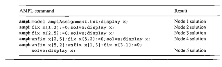
AMPl Moment
Interactive AMPL commands are ideal for the implementation of the TSP B&B algorithm using the general assignment model (file ampIAssignment.txt). The following table summarizes the AMPL commands needed to create the B&B tree in Figure 9.13 (Example 9.3-4):
3 .Cutting-Plane Algorithm
The idea of the cutting plane algorithm is to add a set of constraints to the assignment problem that prevent the formation of a subtour. The additional constraints are defined as follows. In an n-city situation, associate a continuous variable uj (≥ 0) with cities 2, 3, ... , and n. Next, define the required set of additional constraints as

These constraints, when added to the assignment model, will automatically remove all subtour solutions.
Example 9.3-5
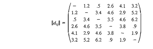
Consider the following distance matrix of a 4-city TSP problem.
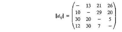
The associated LP consists of the assignment model constraints plus the additional constraints in the table below. All xij = (0, 1) and all uj ≥ 0.
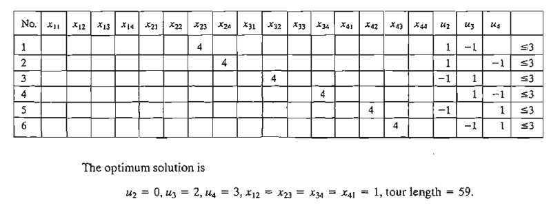
This corresponds to the tour solution 1-2-3-4-1. The solution satisfies all the additional constraints in uj (verify!).
To demonstrate that subtour solutions do not satisfy the additional constraints, consider (1-2-1,3-4-3), which corresponds to x12 = x21 = 1, x34 = x43 = 1. Now, consider constraint 6 in the tableau above:

Substituting x43 = 1, u3 = 2, u4 = 3 yields 5 ≤ 3, which is impossible, thus disallowing x43 = 1 and subtour 3-4-3.
The disadvantage of the cutting-plane model is that the number of variables grows exponentially with the number of cities, making it difficult to obtain a numeric solution for practical situations. For this reason, the B&B algorithm (coupled with the heuristic) may be a more feasible alternative for solving the problem.
AMPL Moment
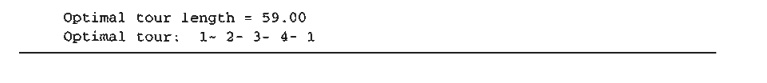
Figure 9.14 provides the AMPL model of the cutting-plane algorithm (file amplEx9.3-5.txt). The data of the 4-cityTSP of Example 9.3-5 are used to drive the model. The for-mulation is straightforward: The fIrst two sets of constraints define the assignment model associated with the problem, and the third set represents the cuts needed to re-move subtour solutions. Notice that the assignment-model variables must be binary and that option solver cplex; must precede solve; to ensure that the obtained so-lution is integer.
The for and if - then statements at the bottom of the model are used to present the out-put in the following readable format:
Related Topics