Branch-and-Bound (B&B) Algorithm

Branch-and-Bound (B&B) Algorithm

The first B&B algorithm was developed in 1960 by A. Land and G. Doig for the general mixed and pure ILP problem. Later, in 1965, E. Balas developed the additive algorithm for solving ILP problems with pure binary (zero or one) variable. The additive algorithm's computations were so simple (mainly addition and subtraction) that it was hailed as a possible breakthrough in the solution of general ILP. Unfortunately, it failed to produce the desired computational advantages. Moreover, the algorithm, which initially appeared unrelated to the B&B technique, was shown to be but a special case of the general Land and Doig algorithm.

This section will present the general Land-Doig B&B algorithm only. A numeric example is used to explain the details.

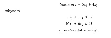
Example 9.2-1

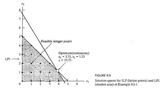
The lattice points (dots) in Figure 9.6 define the ILP solution space. The associated continuous LPI problem at node 1 (shaded area) is defined from ILP by removing the integer restrictions. The optimum solution of LPI is x₁ = 3.75, x₂ = 1.25, and z = 23.75.

Because the optimum LPI solution does not satisfy the integer requirements, the B&B algorithm modifies the solution space in a manner that eventually identifies the ILP optimum. First, we select one of the integer variables whose optimum value at LPI is not integer. Selecting x_l (= 3.75) arbitrarily, the region 3 < x_l < 4 of the LPI solution space contains no integer values of x_1, and thus can be eliminated as nonpromising. This is equivalent to replacing the original LPI with two new LPs:

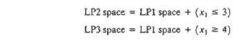
Figure 9.7 depicts the LP2 and LP3 spaces. The two spaces combined contain the same feasible integer points as the original ILP, which means that, from the standpoint of the integer solution, dealing with LP2 and LP3 is the same as dealing with the original LPl; no information is lost.

If we intelligently continue to remove the regions that do not include integer solutions (e.g., 3 < x_l < 4 at LPl) by imposing the appropriate constraints, we will eventually produce LPs whose optimum extreme points satisfy the integer restrictions. In effect, we will be solving the ILP by dealing with a sequence of (continuous) LPs.

The new restrictions, x₁ ≤ 3 and x₁ ≥ 4, are mutually exclusive, so that LP2 and LP3 at nodes 2 and 3 must be dealt with as separate LPs, as Figure 9.8 shows. This dichotomization gives rise to the concept of branching in the B&B algorithm. In this case, x₁ is called the branching variable.

The optimum ILP lies in either LP2 or LP3. Hence, both subproblems must be examined. We arbitrarily examine LP2 (associated with x₁ ≤3) first:

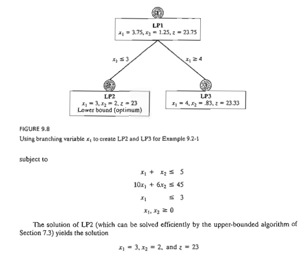
The LP2 solution satisfies the integer requirements for x_l and x₂. Hence, LP2 is said to be fathomed, meaning that it need not be investigated any further because it cannot yield any beller ILP solution.

We cannot at this point say that the integer solution obtained from LP2 is optimum for the original problem, because LP3 may yield a better integer solution with a higher value of z. All we can say is that z = 23 is a lower bound on the optimum (maximum) objective value of the original ILP. This means that any unexamined subproblem that cannot yield a better objective value than the lower bound must be discarded as nonpromising. If an unexamined subproblem produces a better integer solution, then the lower bound must be updated accordingly.

Given the lower bound z = 23, we examine LP3 (the only remaining unexamined subproblem at this point). Because optimum z = 23.75 at LPI and all the coefficients of the objective function happen to be integers, it is impossible that LP3 (which is more restrictive than LPl) will produce a better integer solution with z > 23. As a result, we discard LP3 and conclude that it has been fathomed.

The B&B algorithm is now complete because both LP2 and LP3 have been examined and fathomed (the first for producing an integer solution and the second for failing to produce a better integer solution). We thus conclude that the optimum ILP solution is the one associated with the lower bound-namely, x₁ = 3, x₂, and z = 23.

Two questions remain unanswered regarding the procedure.

a)     At LPI, could we have selected x₂ as the branching variable in place of x_l?

b)    When selecting the next subproblem to be examined, could we have solved LP3 first in-stead of LP2?

The answer to both questions is "yes," but ensuing computations could differ dramatically. Figure 9.9 demonstrates this point. Suppose that we examine LP3 first (instead of LP2 as we did in Figure 9.8). The solution is x_I = 4, x₂ = .83, and z = 23.33 (verify!). Because x₂ (= .83) is noninteger, LP3 is examined further by creating subproblems LP4 and LPS using the branches x₂ ≤ 0 and x2 ≥ 1, respectively. This means that

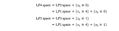
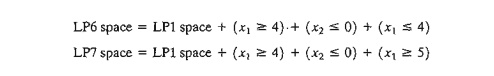
We now have three "dangling" subproblems to be examined: LP2, LP4, and LP5. Suppose that we arbitrarily examine LP5 first. LP5 has no solution, and hence it is fathomed. Next, let us examine LP4. The optimum solution is x_l = 4.5, x₂ = 0, and z = 22.5. The noninteger value of x₁ leads to the two branches x₁ ≤ 4 and X_l ≥ 5, and the creation of subproblems LP6 and LP7 from LP4.

Now, subproblems LP2, LP6, and LP7 remain unexamined. Selecting LP7 for examination, the problem has no feasible solution, and thus is fathomed. Next, we select LP6. The problem yields the first integer solution (x_l = 4, x₂ = 0, z = 20), and thus provides the first lower bound

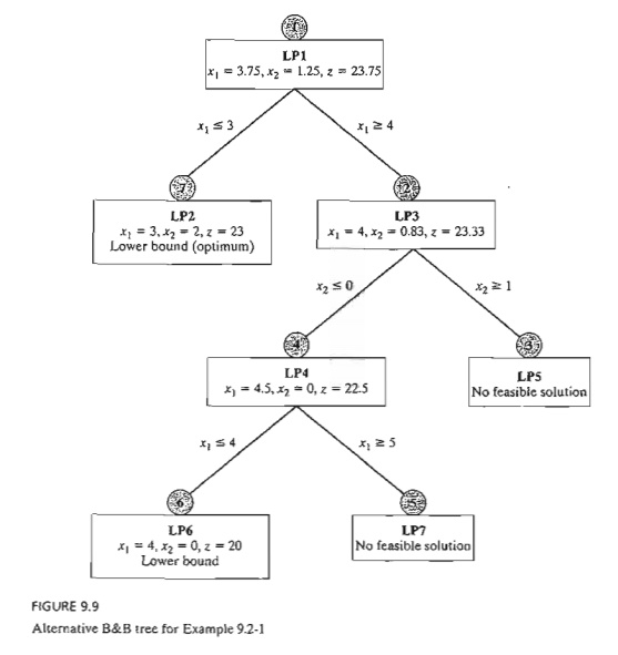
(= 20) on the optimum ILP objective value. We are now left with subproblem LP2, which yields a better integer solution (x₁ = 3, x₂ = 2, z = 23). Thus, the lower bound is updated from z = 20 to z = 23. At this point, all the subproblems have been fathomed (examined) and the optimum solution is the one associated with the most up-to-date lower bound-namely, x_l = 3, x₂ = 2, and z = 23.

The solution sequence in Figure 9.9 (LPl --> LP3 --> LP5 --> LP4 --> LP7 --> LP6 --> LP2) is a worst-case scenario that, nevertheless, may well occur in practice. In Figure 9.8, we were lucky to "stumble" upon a good lower bound at the very first subproblem we examined (LP2), thus allowing us to fathom LP3 without investigating it. In essence, we compieted the procedure by solving a total of two LPs. In Figure 9.9, the story is different: We needed to solve seven LPs before the B&B algo-rithm could be terminated.

Remarks. The example points to a principal weakness in the B&B algorithm: Given multiple choices, how do we select the next subproblem and its branching variable? Although there are heuristics for enhancing the ability of B&B to "foresee" which branch can lead to an improved ILP solution (see Taha, 1975, pp. 154-171), solid theory with consistent results does not exist, and herein lies the difficulty that plagues computations in ILP. Indeed, Problem 7, Set 9.2a, demonstrates the bizarre behavior of the B&B algorithm in investigating over 25,000 LPs before optimality is verified, even though the problem is quite small (16 binary variables and 1 constraint). Unfortunately, to date, and after more than four decades of research coupled with tremendous advances in computing power, available ILP codes (commercial and academic alike) are not to-tally reliable, in the sense that they may not find the optimum ILP solution regardless of how long they execute on the computer. What is even more frustrating is that this behavior can apply just the same to some relatively small problems.

AMPL Moment

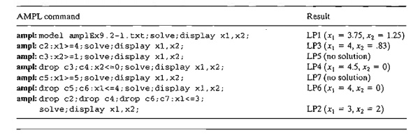
AMPL can be used interactively to generate the B&B search tree. The following table shows the sequence of commands needed to generate the tree of Example 9.2-1 (Figure 9.9) starting with the continuous LPO. AMPL model (file ampIEx9.2-1.txt) has two variables x_l and x₂ and two constraints c₀ and c_l. You will find it helpful to synchronize the AMPL commands with the branches in Figure 9.9.

Solver Moment

Solver can be used to obtain the solution of the different subproblems by using the add/change/delete options in the Solver Parameters dialogue box.

Summary of the B&B Algorithm. We now summarize the B&B algorithm. Assuming a maximization problem, set an initial lower bound z = - ¥ on the optimum objective value of ILP. Set i = 0.

Step 1. (Fathoming/bounding). Select LPi, the next subproblem to be examined. Solve LPi, and attempt to fathom it using one of three conditions:

a)   The optimal z-value of LPi cannot yield a better objective value than the current lower bound.

b)   LPi yields a better feasible integer solution than the current lower bound.

c)     LPi has no feasible solution.

Two cases will arise.

a)     If LPi is fathomed and a better solution is found, update the lower bound. If all subproblems have been fathomed, stop; the optimum ILP is associated with the current finite lower bound. If no finite lower bound exists, the problem has no feasible solution. Else, set i = i + 1, and repeat step 1.

b)    If LPi is not fathomed, go to step 2 for branching.

Step 2. (Branching). Select one of the integer variables x_j, whose optimum value x_j* in the LPi solution is not integer. Eliminate the region

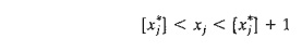
(where [v] defines the largest integer ≤ v) by creating two LP subproblems that correspond to

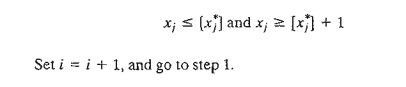
The given steps apply to maximization problems. For minimization, we replace the lower bound with an upper bound (whose initial value is z = +¥).

The B&B algorithm can be extended directly to mixed problems (in which only some of the variables are integer). If a variable is continuous, we simply never select it as a branching variable. A feasible subproblem provides a new bound on the objective value if the values of the discrete variables are integer and the objective value is improved relative to the current bound.

PROBLEM SET 9.2A

1.      Solve the ILP of Example 9.2-1 by the B&B algorithm starting with X₂ as the branching variable. Start the procedure by solving the subproblem associated with X₂ ≤ [x₂*].

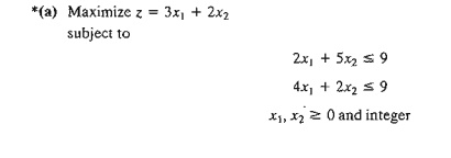
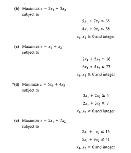
2.      Develop the B&B tree for each of the following problems. For convenience, always select X_l as the branching variable at node 0.

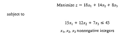
7. TO RA/Solver / AMPL Experiment. The following problem is designed to demonstrate the bizarre behavior of the B&B algorithm even for small problems. In particular, note how many subproblems are examined before the optimum is found and how many are needed to verify optimality.

a)      Use TORA's automated option to show that although the optimum is found after only 9 subproblems, over 25,000 subproblems are examined before optimality is confirmed.

b)      Show that Solver exhibits an experience similar to TORA's. [Note: In Solver, you can watch the change in the number of generated branches (subproblems) at the bottom of the spreadsheet.]

c)      Solve the problem with AMPL and show that the solution is obtained instantly with oMIP simplex iterations and 0 B&B nodes. The reason for this superior perfor-mance can only be attributed to preparatory steps performed by AMPL and/or the CPLEX solver prior to solving the problem.

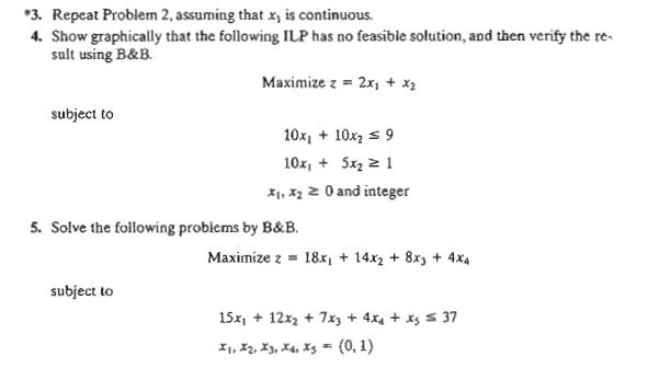
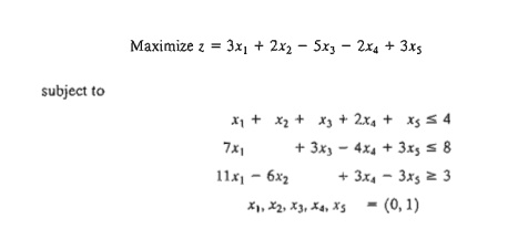
8. TORA Experiment. Consider the following ILP:

Use TORA's B&B user-guided option to generate the search tree with and without acti-vating the objective-value bound. What is the impact of activating the objective-value bound on the number of generated subproblems? For consistency, always select the branching variable as the one with the lowest index and investigate all the subproblems in a current row from left to right before moving to the next row.

*9. TORA Experiment. Reconsider Problem 8 above. Convert the problem into an equivalent 0-1 ILP, then solve it with TORA's automated option. Compare the size of the search trees in the two problems.

10. AMPL Experiment. In the following 0-1 ILP use interactive AMPL to generate the asso-ciated search tree. In each case, show how the z-bound is used to fathom subproblems.