The Distribution of Measurements and Results

The Distribution of Measurements and Results

An analysis, particularly a quantitative analysis, is usually performed on several replicate samples. How do we report the result for such an experiment when results for the replicates are scattered around a central value? To complicate matters fur- ther, the analysis of each replicate usually requires multiple measurements that, themselves, are scattered around a central value.

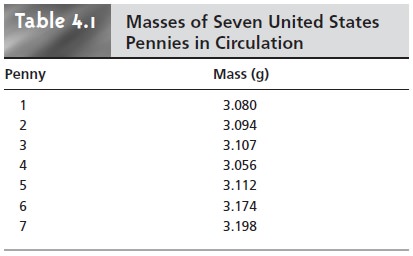
Consider, for example, the data in Table 4.1 for the mass of a penny. Reporting only the mean is insufficient because it fails to indicate the uncertainty in measuring a penny’s mass. Including the standard deviation, or other measure of spread, pro- vides the necessary information about the uncertainty in measuring mass. Never- theless, the central tendency and spread together do not provide a definitive state- ment about a penny’s true mass. If you are not convinced that this is true, ask yourself how obtaining the mass of an additional penny will change the mean and standard deviation.

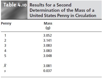
How we report the result of an experiment is further complicated by the need to compare the results of different experiments. For example, Table 4.10 shows re- sults for a second, independent experiment to determine the mass of a U.S. penny in circulation. Although the results shown in Tables 4.1 and 4.10 are similar, they are not identical; thus, we are justified in asking whether the results are in agree- ment. Unfortunately, a definitive comparison between these two sets of data is not possible based solely on their respective means and standard deviations.

Developing a meaningful method for reporting an experiment’s result requires the ability to predict the true central value and true spread of the population under investigation from a limited sampling of that population. In this section we will take a quantitative look at how individual measurements and results are distributed around a central value.

Populations and Samples

In the previous section we introduced the terms “population” and “sample” in the context of reporting the result of an experiment. Before continuing, we need to un- derstand the difference between a population and a sample. A population is the set of all objects in the system being investigated. These objects, which also are mem- bers of the population, possess qualitative or quantitative characteristics, or values, that can be measured. If we analyze every member of a population, we can deter- mine the population’s true central value, μ, and spread, σ.

The probability of occurrence for a particular value, P(V), is given as

where V is the value of interest, M is the value’s frequency of occurrence in the pop- ulation, and N is the size of the population. In determining the mass of a circulating United States penny, for instance, the members of the population are all United States pennies currently in circulation, while the values are the possible masses that a penny may have.

In most circumstances, populations are so large that it is not feasible to analyze every member of the population. This is certainly true for the population of circulating U.S. pennies. Instead, we select and analyze a limited subset, or sample, of the popula- tion. The data in Tables 4.1 and 4.10, for example, give results for two samples drawn at random from the larger population of all U.S. pennies currently in circulation.

Probability Distributions for Populations

To predict the properties of a population on the basis of a sample, it is necessary to know something about the population’s expected distribution around its central value. The distribution of a population can be represented by plotting the frequency of occurrence of individual values as a function of the values themselves. Such plots are called probability distributions. Unfortunately, we are rarely able to calculate the exact probability distribution for a chemical system. In fact, the probability dis- tribution can take any shape, depending on the nature of the chemical system being investigated. Fortunately many chemical systems display one of several common probability distributions. Two of these distributions, the binomial distribution and the normal distribution, are discussed next.

Binomial Distribution 

The binomial distribution describes a population in which the values are the number of times a particular outcome occurs during a fixed num- ber of trials. Mathematically, the binomial distribution is given as

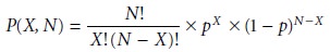
where P(X,N) is the probability that a given outcome will occur X times during N trials, and p is the probability that the outcome will occur in a single trial.* If you flip a coin five times, P(2,5) gives the probability that two of the five trials will turn up “heads.”

A binomial distribution has well-defined measures of central tendency and spread. The true mean value, for example, is given as

μ = Np

and the true spread is given by the variance

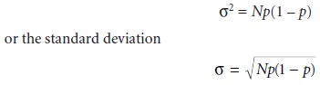
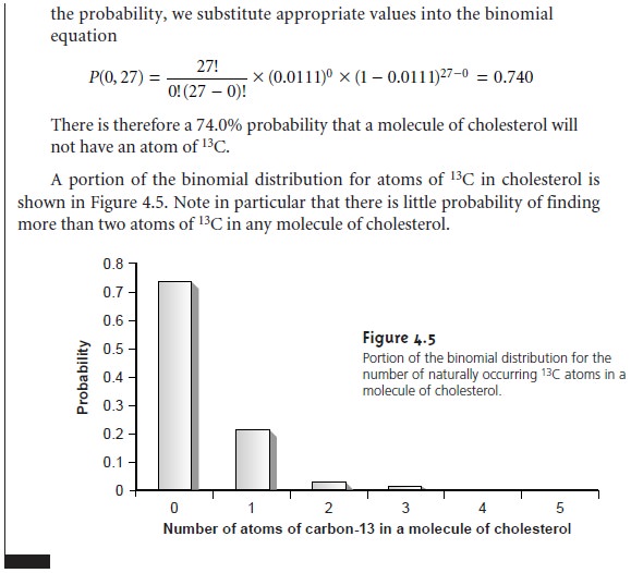
The binomial distribution describes a population whose members have only certain, discrete values. A good example of a population obeying the binomial dis- tribution is the sampling of homogeneous materials. As shown in Example 4.10, the binomial distribution can be used to calculate the probability of finding a particular isotope in a molecule.

Normal Distribution 

The binomial distribution describes a population whose members have only certain, discrete values. This is the case with the number of 13C atoms in a molecule, which must be an integer number no greater then the number of carbon atoms in the molecule. A molecule, for example, cannot have 2.5 atoms of 13C. Other populations are considered continuous, in that members of the popula- tion may take on any value.

The most commonly encountered continuous distribution is the Gaussian, or normal distribution, where the frequency of occurrence for a value, X, is given by

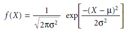
The shape of a normal distribution is determined by two parameters, the first of which is the population’s central, or true mean value, μ, given as

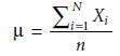
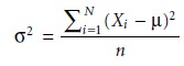
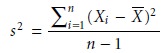
where n is the number of members in the population. The second parameter is the population’s variance, σ2, which is calculated using the following equation*

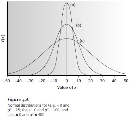
Examples of normal distributions with μ = 0 and σ2 = 25, 100 or 400, are shown in Figure 4.6. Several features of these normal distributions deserve atten- tion. First, note that each normal distribution contains a single maximum corre- sponding to μ and that the distribution is symmetrical about this value. Second, increasing the population’s variance increases the distribution’s spread while de- creasing its height. Finally, because the normal distribution depends solely on μ and σ2, the area, or probability of occurrence between any two limits defined in terms of these parameters is the same for all normal distribution curves. For ex- ample, 68.26% of the members in a normally distributed population have values within the range μ ±1σ, regardless of the actual values of μ and σ. As shown in Example 4.11, probability tables (Appendix 1A) can be used to determine the probability of occurrence between any defined limits.

Confidence Intervals for Populations

If we randomly select a single member from a pop- ulation, what will be its most likely value? This is an important question, and, in one form or another, it is the fundamental problem for any analysis. One of the most important features of a population’s probability distribution is that it provides a way to answer this question.

Earlier we noted that 68.26% of a normally distrib- uted population is found within the range of μ ± 1σ. Stat- ing this another way, there is a 68.26% probability that a member selected at random from a normally distributed population will have a value in the interval of μ ± 1σ. In general, we can write

X_i =  =μ± zσ      ------------- 4.9

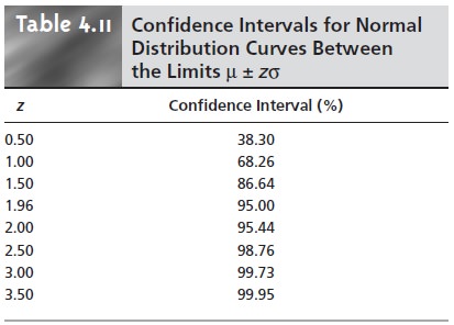
where the factor z accounts for the desired level of confidence. Values reported in this fashion are called confidence intervals. Equation 4.9, for example, is the confidence interval for a single member of a population. Confidence intervals can be quoted for any desired probability level, several examples of which are shown in Table 4.11. For reasons that will be discussed later, a 95% confidence interval frequently is reported.

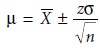
Alternatively, a confidence interval can be expressed in terms of the popula- tion’s standard deviation and the value of a single member drawn from the popu- lation. Thus, equation 4.9 can be rewritten as a confidence interval for the population mean

                 4. 10

Confidence intervals also can be reported using the mean for a sample of size n, drawn from a population of known σ. The standard deviation for the mean value, σx’, which also is known as the standard error of the mean, is

Probability Distributions for Samples

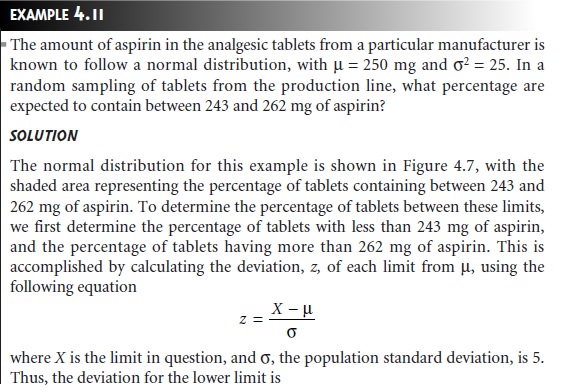
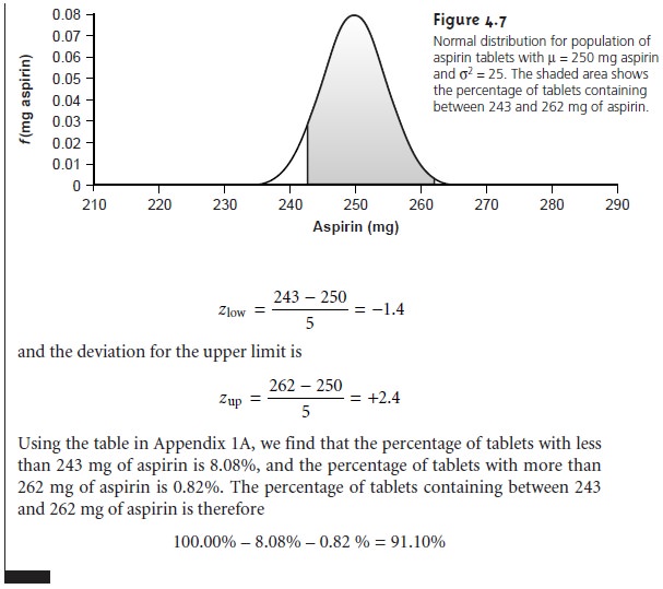
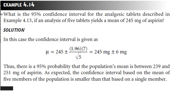
We introduced two probability distributions commonly encoun- tered when studying populations. The construction of confidence intervals for a normally distributed population. We have yet to ad- dress, however, how we can identify the probability distribution for a given popula- tion. In Examples 4.11–4.14 we assumed that the amount of aspirin in analgesic tablets is normally distributed. We are justified in asking how this can be deter- mined without analyzing every member of the population. When we cannot study the whole population, or when we cannot predict the mathematical form of a popu- lation’s probability distribution, we must deduce the distribution from a limited sampling of its members.

Sample Distributions and the Central Limit Theorem 

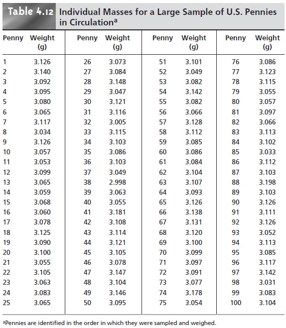
Let’s return to the problem of determining a penny’s mass to explore the relationship between a population’s distribution and the distribution of samples drawn from that population. The data shown in Tables 4.1 and 4.10 are insufficient for our purpose because they are not large enough to give a useful picture of their respective probability distributions. A better picture of the probability distribution requires a larger sample, such as that shown in Table 4.12, for which X– is 3.095 and s² is 0.0012.

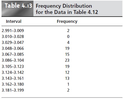
The data in Table 4.12 are best displayed as a histogram, in which the fre- quency of occurrence for equal intervals of data is plotted versus the midpoint of each interval. Table 4.13 and Figure 4.8 show a frequency table and histogram for the data in Table 4.12. Note that the histogram was constructed such that the mean value for the data set is centered within its interval. In addition, a normal distribution curve using X– and s to estimate μ and σ is superimposed on the histogram.

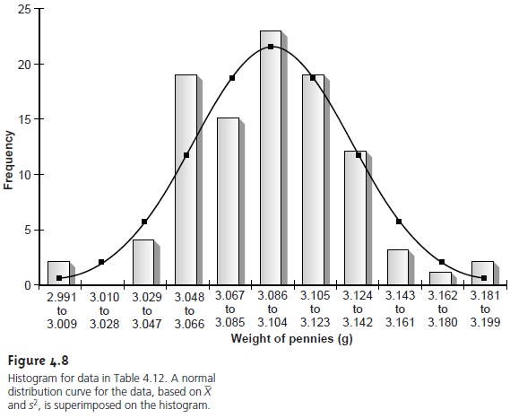
It is noteworthy that the histogram in Figure 4.8 approximates the normal dis- tribution curve. Although the histogram for the mass of pennies is not perfectly symmetrical, it is roughly symmetrical about the interval containing the greatest number of pennies. In addition, we know from Table 4.11 that 68.26%, 95.44%, and 99.73% of the members of a normally distributed population are within, re- spectively, ±1σ, ±2σ and ±3σ. If we assume that the mean value, 3.095 g, and the sample variance, 0.0012, are good approximations for μ and σ2, we find that 73%, 95%, and 100% of the pennies fall within these limits. It is easy to imagine that in- creasing the number of pennies in the sample will result in a histogram that even more closely approximates a normal distribution.

We will not offer a formal proof that the sample of pennies in Table 4.12 and the population from which they were drawn are normally distributed; how- ever, the evidence we have seen strongly suggests that this is true. Although we cannot claim that the results for all analytical experiments are normally distrib- uted, in most cases the data we collect in the laboratory are, in fact, drawn from a normally distributed population. That this is generally true is a consequence of the central limit theorem. According to this theorem, in systems subject to a variety of indeterminate errors, the distribution of results will be approximately normal. Furthermore, as the number of contributing sources of indeterminate error increases, the results come even closer to approximating a normal distribu- tion. The central limit theorem holds true even if the individual sources of in- determinate error are not normally distributed. The chief limitation to the central limit theorem is that the sources of indeterminate error must be indepen- dent and of similar magnitude so that no one source of error dominates the final distribution.

Estimating μ and σ2 

Our comparison of the histogram for the data in Table 4.12 to a normal distribution assumes that the sample’s mean, X–, and variance, s² , are appropriate estimators of the population’s mean, μ, and variance, σ2. Why did we select X– and s² , as opposed to other possible measures of central tendency and spread? The explanation is simple; X– and s² are considered unbiased estimators of μ and σ2.If we could analyze every possible sample of equal size for a given popula- tion (e.g., every possible sample of five pennies), calculating their respective means and variances, the average mean and the average variance would equal μ and σ2. Al- though X– and s² for any single sample probably will not be the same as μ or σ² , they provide a reasonable estimate for these values.

Degrees of Freedom 

Unlike the population’s variance, the variance of a sample in- cludes the term n – 1 in the denominator, where n is the size of the sample

                   4.12

Defining the sample’s variance with a denominator of n, as in the case of the popu- lation’s variance leads to a biased estimation of x2. The denominators of the vari- ance equations 4.8 and 4.12 are commonly called the degrees of freedom for the population and the sample, respectively. In the case of a population, the degrees of freedom is always equal to the total number of members, n, in the population. For the sample’s variance, however, substituting X for μ removes a degree of freedom from the calculation. That is, if there are n members in the sample, the value of the nth member can always be deduced from the remaining n – 1 members and X–. For example, if we have a sample with five members, and we know that four of the members a re 1, 2, 3, and 4, and that the mean is 3, then the fifth member of the sample must be

(X– x n)– X₁ – X₂ – X₃ – X₄ = (3 x 5)–1–2–3–4=5

Confidence Intervals for Samples

Earlier we introduced the confidence interval as a way to report the most probable value for a population’s mean, μ, when the population’s standard deviation, σ , is known. Since s2 is an unbiased estimator of σ 2, it should be possible to construct confidence intervals for samples by replacing  in equations 4.10 and 4.11 with s. Two complications arise, however. The first is that we cannot define s2 for a single member of a population. Consequently, equation 4.10 cannot be extended to situa- tions in which s2 is used as an estimator of  s2. In other words, when e is unknown, we cannot construct a confidence interval for μ by sampling only a single member of the population.

The second complication is that the values of z shown in Table 4.11 are derived for a normal distribution curve that is a function of σ 2, not s2. Although s2 is an  unbiased  estimator of  σ 2, the value of  s2 for any randomly selected sample may differ significantly from   σ2. To account for the uncertainty in estimating  σ 2, the term  z  in equation 4.11 is replaced with the variable t, where t is defined such that t >= z at all confidence levels. Thus, equation 4.11 becomes

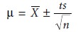                   4.13

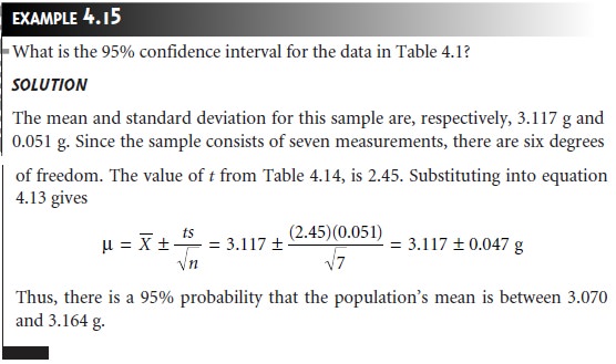
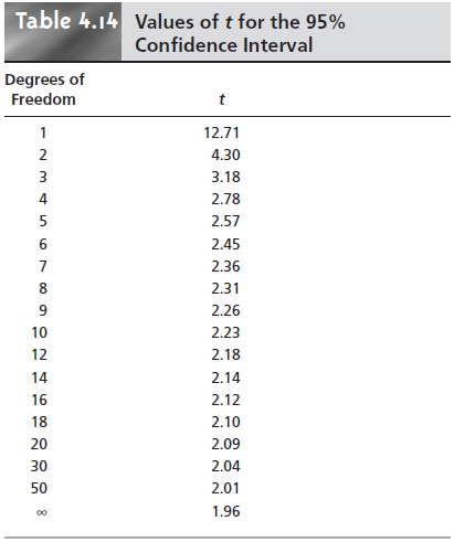
Values for t at the 95% confidence level are shown in Table 4.14. Note that t be- comes smaller as the number of the samples (or degrees of freedom) increase, ap- proaching z as n approaches infinity. Additional values of t for other confidence lev- els can be found in Appendix 1B.

A Cautionary Statement

There is a temptation when analyzing data to plug numbers into an equation, carry out the calculation, and report the result. This is never a good idea, and you should develop the habit of constantly reviewing and evaluating your data. For example, if analyzing five samples gives an analyte’s mean concentration as 0.67 ppm with a standard deviation of 0.64 ppm, then the 95% confidence interval  is

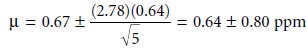
This confidence interval states that the analyte’s true concentration lies within the range of –0.16 ppm to 1.44 ppm. Including a negative concentration within the con- fidence interval should lead you to reevaluate your data or conclusions. On further investigation your data may show that the standard deviation is larger than expected, making the confidence interval too broad, or you may conclude that the analyte’s concentration is too small to detect accurately.*

A second example is also informative. When samples are obtained from a nor- mally distributed population, their values must be random. If results for several samples show a regular pattern or trend, then the samples cannot be normally dis- tributed. This may reflect the fact that the underlying population is not normally distributed, or it may indicate the presence of a time-dependent determinate error. For example, if we randomly select 20 pennies and find that the mass of each penny exceeds that of the preceding penny, we might suspect that the balance on which the pennies are being weighed is drifting out of calibration.