Analytical Data: Characterizing Experimental Errors

Characterizing Experimental Errors

Realizing that our data for the mass of a penny can be characterized by a measure of central tendency and a measure of spread suggests two questions. First, does our measure of central tendency agree with the true, or expected value? Second, why are our data scattered around the central value? Errors associated with central tendency reflect the accuracy of the analysis, but the precision of the analysis is determined by those errors associated with the spread.

Accuracy

Accuracy is a measure of how close a measure of central tendency is to the true, or expected value, μ.† Accuracy is usually expressed as either an absolute error

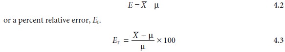
Although the mean is used as the measure of central tendency in equations 4.2 and 4.3, the median could also be used.

Errors affecting the accuracy of an analysis are called determinate and are char- acterized by a systematic deviation from the true value; that is, all the individual measurements are either too large or too small. A positive determinate error results in a central value that is larger than the true value, and a negative determinate error leads to a central value that is smaller than the true value. Both positive and nega- tive determinate errors may affect the result of an analysis, with their cumulative ef- fect leading to a net positive or negative determinate error. It is possible, although not likely, that positive and negative determinate errors may be equal, resulting in a central value with no net determinate error.

Determinate errors may be divided into four categories: sampling errors, method errors, measurement errors, and personal errors.

Sampling Errors 

We introduce determinate sampling errors when our sampling strategy fails to provide a representative sample. This is especially important when sampling heterogeneous materials. For example, determining the environmental quality of a lake by sampling a single location near a point source of pollution, such as an outlet for industrial effluent, gives misleading results. In determining the mass of a U.S. penny, the strategy for selecting pennies must ensure that pennies from other countries are not inadvertently included in the sample.

Method Errors 

Determinate method errors are introduced when assumptions about the relationship between the signal and the analyte are invalid. In terms of the general relationships between the measured signal and the amount of analyte

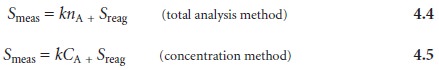
method errors exist when the sensitivity, k, and the signal due to the reagent blank, S_reag, are incorrectly determined. For example, methods in which S_meas is the mass of a precipitate containing the analyte (gravimetric method) assume that the sensitiv- ity is defined by a pure precipitate of known stoichiometry. When this assumption fails, a determinate error will exist. Method errors involving sensitivity are mini- mized by standardizing the method, whereas method errors due to interferents present in reagents are minimized by using a proper reagent blank. Method errors due to interferents in the sample cannot be minimized by a reagent blank. Instead, such interferents must be sepa- rated from the analyte or their concentrations determined independently.

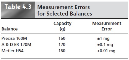
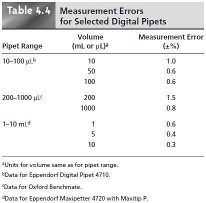
Measurement Errors 

Analytical instruments and equipment, such as glassware and balances, are usually supplied by the manufacturer with a statement of the item’s maximum measurement error, or tolerance. For example, a 25-mL volumetric flask might have a maximum error of ±0.03 mL, meaning that the actual volume contained by the flask lies within the range of 24.97–25.03 mL. Although expressed as a range, the error is determinate; thus, the flask’s true volume is a fixed value within the stated range. A summary of typical measurement errors for a variety of analytical equipment is given in Tables 4.2–4.4.

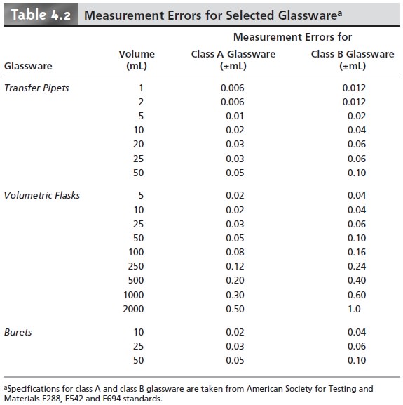
Volumetric glassware is categorized by class. Class A glassware is manufactured to comply with tolerances specified by agencies such as the National Institute of Standards and Technology. Tolerance levels for class A glassware are small enough that such glassware normally can be used without calibration. The tolerance levels for class B glassware are usually twice those for class A glassware. Other types of vol- umetric glassware, such as beakers and graduated cylinders, are unsuitable for accu- rately measuring volumes.

Determinate measurement errors can be minimized by calibration. A pipet can be calibrated, for example, by determining the mass of water that it delivers and using the density of water to calculate the actual volume delivered by the pipet. Al- though glassware and instrumentation can be calibrated, it is never safe to assume that the calibration will remain unchanged during an analysis. Many instruments, in particular, drift out of calibration over time. This complication can be minimized by frequent recalibration.

Personal Errors 

Finally, analytical work is always subject to a variety of personal errors, which can include the ability to see a change in the color of an indicator used to signal the end point of a titration; biases, such as consistently overestimat- ing or underestimating the value on an instrument’s readout scale; failing to cali- brate glassware and instrumentation; and misinterpreting procedural directions. Personal errors can be minimized with proper care.

Identifying Determinate Errors 

Determinate errors can be difficult to detect. Without knowing the true value for an analysis, the usual situation in any analysis with meaning, there is no accepted value with which the experimental result can be compared. Nevertheless, a few strategies can be used to discover the presence of a determinate error.

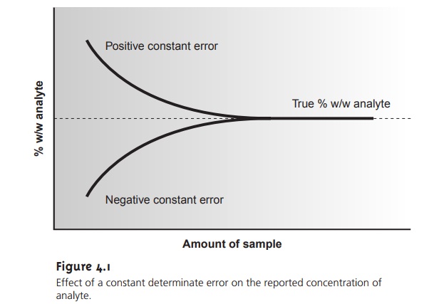
Some determinate errors can be detected experimentally by analyzing several samples of different size. The magnitude of a constant determinate error is the same for all samples and, therefore, is more significant when analyzing smaller sam- ples. The presence of a constant determinate error can be detected by running sev- eral analyses using different amounts of sample, and looking for a systematic change in the property being measured. For example, consider a quantitative analysis in which we separate the analyte from its matrix and determine the analyte’s mass. Let’s assume that the sample is 50.0% w/w analyte; thus, if we analyze a 0.100-g sample, the analyte’s true mass is 0.050 g. The first two columns of Table 4.5 give the true mass of analyte for several additional samples. If the analysis has a positive constant determinate error of 0.010 g, then the experimentally determined mass for

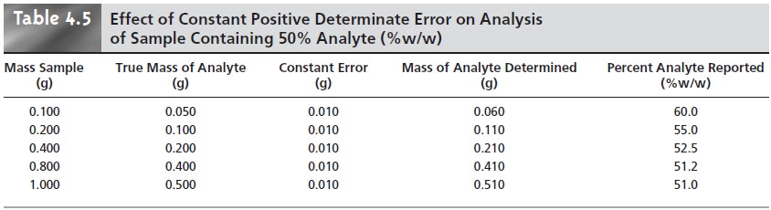
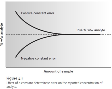
any sample will always be 0.010 g, larger than its true mass (column four of Table 4.5). The analyte’s reported weight percent, which is shown in the last column of Table 4.5, becomes larger when we analyze smaller samples. A graph of % w/w ana- lyte versus amount of sample shows a distinct upward trend for small amounts of sample (Figure 4.1). A smaller concentration of analyte is obtained when analyzing smaller samples in the presence of a constant negative determinate error.

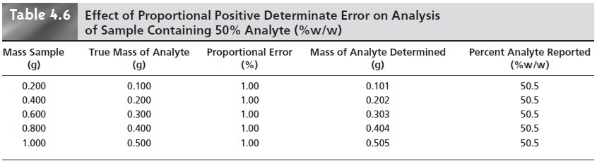
A proportional determinate error, in which the error’s magnitude depends on the amount of sample, is more difficult to detect since the result of an analysis is in- dependent of the amount of sample. Table 4.6 outlines an example showing the ef- fect of a positive proportional error of 1.0% on the analysis of a sample that is 50.0% w/w in analyte. In terms of equations 4.4 and 4.5, the reagent blank, S_reag, is an example of a constant determinate error, and the sensitivity, k, may be affected by proportional errors.

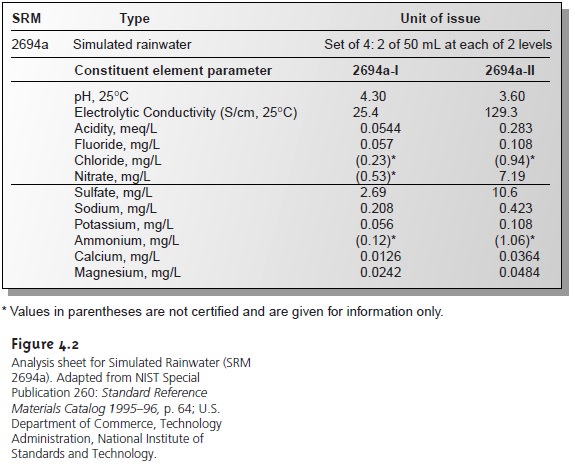
Potential determinate errors also can be identified by analyzing a standard sam- ple containing a known amount of analyte in a matrix similar to that of the samples being analyzed. Standard samples are available from a variety of sources, such as the National Institute of Standards and Technology (where they are called standard reference materials) or the American Society for Testing and Materials. For exam- ple, Figure 4.2 shows an analysis sheet for a typical reference material. Alternatively, the sample can be analyzed by an independent method known to give accurate results, and the re- sults of the two methods can be compared. Once identified, the source of a determinate error can be corrected. The best prevention against errors affect- ing accuracy, however, is a well-designed procedure that identifies likely sources of determinate errors, coupled with careful laboratory work.

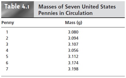
The data in Table 4.1 were obtained using a calibrated balance, certified by the manufacturer to have a tolerance of less than ±0.002 g. Suppose the Treasury Department reports that the mass of a1998 U.S. penny is approximately 2.5 g. Since the mass of every penny in Table 4.1 exceeds the re- ported mass by an amount significantly greater than the balance’s tolerance, we can safely conclude that the error in this analysis is not due to equip- ment error.

Precision

Precision is a measure of the spread of data about a central value and may be ex- pressed as the range, the standard deviation, or the variance. Precision is commonly divided into two categories: repeatability and reproducibility. Repeatability is the precision obtained when all measurements are made by the same analyst during a single period of laboratory work, using the same solutions and equipment. Repro- ducibility, on the other hand, is the precision obtained under any other set of con- ditions, including that between analysts, or between laboratory sessions for a single analyst. Since reproducibility includes additional sources of variability, the repro- ducibility of an analysis can be no better than its repeatability.

Errors affecting the distribution of measurements around a central value are called indeterminate and are characterized by a random variation in both magni- tude and direction. Indeterminate errors need not affect the accuracy of an analy- sis. Since indeterminate errors are randomly scattered around a central value, posi- tive and negative errors tend to cancel, provided that enough measurements are made. In such situations the mean or median is largely unaffected by the precision of the analysis.

Sources of Indeterminate Error 

Indeterminate errors can be traced to several sources, including the collection of samples, the manipulation of samples during the analysis, and the making of measurements.

When collecting a sample, for instance, only a small portion of the available material is taken, increasing the likelihood that small-scale inhomogeneities in the sample will affect the repeatability of the analysis. Individual pennies, for example, are expected to show variation from several sources, including the manufacturing process, and the loss of small amounts of metal or the addition of dirt during circu- lation. These variations are sources of indeterminate error associated with the sam- pling process.

During the analysis numerous opportunities arise for random variations in the way individual samples are treated. In determining the mass of a penny, for exam- ple, each penny should be handled in the same manner. Cleaning some pennies but not cleaning others introduces an indeterminate error.

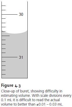
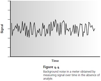
Finally, any measuring device is subject to an indeterminate error in reading its scale, with the last digit always being an estimate subject to random fluctuations, or background noise. For example, a buret with scale divisions every 0.1 mL has an in- herent indeterminate error of ±0.01 – 0.03 mL when estimating the volume to the hundredth of a milliliter (Figure 4.3). Background noise in an electrical meter (Figure 4.4) can be evaluated by recording the signal without analyte and observing the fluctuations in the signal over time.

Evaluating Indeterminate Error 

Although it is impossible to eliminate indetermi- nate error, its effect can be minimized if the sources and relative magnitudes of the indeterminate error are known. Indeterminate errors may be estimated by an ap- propriate measure of spread. Typically, a standard deviation is used, although in some cases estimated values are used. The contribution from analytical instruments and equipment are easily measured or estimated. Inde- terminate errors introduced by the analyst, such as in- consistencies in the treatment of individual samples, are more difficult to estimate.

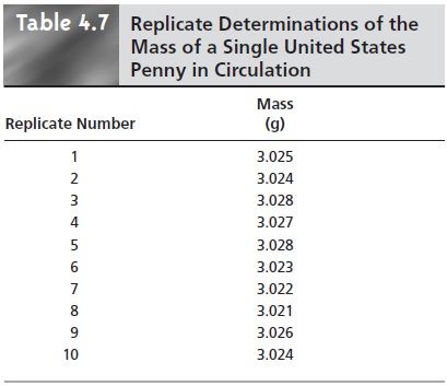
To evaluate the effect of indeterminate error on the data in Table 4.1, ten replicate determinations of the mass of a single penny were made, with results shown in Table 4.7. The standard deviation for the data in Table 4.1 is 0.051, and it is 0.0024 for the data in Table 4.7. The significantly better precision when determining the mass of a single penny sug- gests that the precision of this analysis is not limited by the balance used to measure mass, but is due to a significant variability in the masses of individual pennies.

Error and Uncertainty

Analytical chemists make a distinction between error and uncertainty.3 Error is the difference between a single measurement or result and its true value. In other words, error is a measure of bias. As discussed earlier, error can be divided into de- terminate and indeterminate sources. Although we can correct for determinate error, the indeterminate portion of the error remains. Statistical significance testing, provides a way to determine whether a bias resulting from determinate error might be present.

Uncertainty expresses the range of possible values that a measurement or result might reasonably be expected to have. Note that this definition of uncertainty is not the same as that for precision. The precision of an analysis, whether reported as a range or a standard deviation, is calculated from experimental data and provides an estimation of indeterminate error affecting measurements. Uncertainty accounts for all errors, both determinate and indeterminate, that might affect our result. Al- though we always try to correct determinate errors, the correction itself is subject to random effects or indeterminate errors.

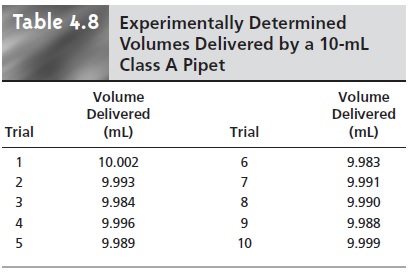
To illustrate the difference between precision and un- certainty, consider the use of a class A 10-mL pipet for de- livering solutions. A pipet’s uncertainty is the range of volumes in which its true volume is expected to lie. Sup- pose you purchase a 10-mL class A pipet from a labora- tory supply company and use it without calibration. The pipet’s tolerance value of ±0.02 mL (see Table 4.2) repre- sents your uncertainty since your best estimate of its vol- ume is 10.00 mL ±0.02 mL. Precision is determined ex- perimentally by using the pipet several times, measuring the volume of solution delivered each time. Table 4.8 shows results for ten such trials that have a mean of 9.992 mL and a standard deviation of 0.006. This standard devi- ation represents the precision with which we expect to be able to deliver a given solution using any class A 10-mL pipet. In this case the uncertainty in using a pipet is worse than its precision. Interestingly, the data in Table 4.8 allow us to calibrate this specific pipet’s delivery volume as 9.992 mL. If we use this vol- ume as a better estimate of this pipet’s true volume, then the uncertainty is ±0.006. As expected, calibrating the pipet allows us to lower its uncertainty.