Statistical Methods for Normal Distributions

Statistical Methods for Normal Distributions

The most commonly encountered probability distribution is the normal, or Gaussian, distribution. A normal distribution is characterized by a true mean, μ, and variance σ², which are estimated using X– and s . Since the area between any two limits of a normal distribution is well defined, the construction and evaluation of significance tests are straightforward.

Comparing X– to μ

One approach for validating a new analytical method is to analyze a standard sample containing a known amount of analyte, μ. The method’s accuracy is judged by determining the average amount of analyte in several samples, X, and using a significance test to compare it with μ The null hypothesis is that X andμ are the same and that any difference between the two values can be explained by in-

 determinate errors affecting the determination of X–. The alternative hypothesis is that the difference between  X– and μ is too large to be explained by indeterminate error.

The equation for the test (experimental) statistic, t_exp, is derived from the confi- dence interval for μ

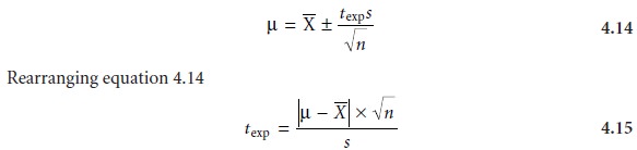
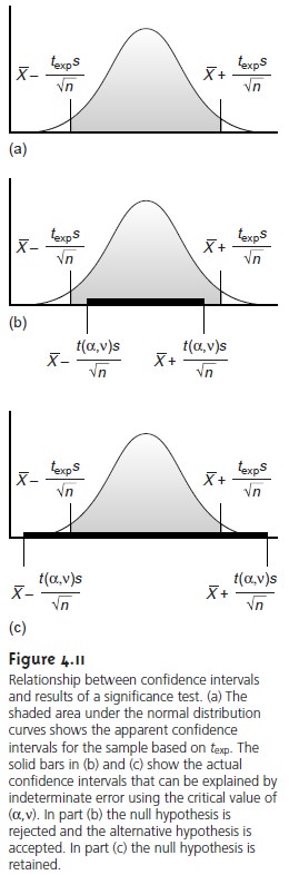
gives the value of t_exp when μ is at either the right or left edge of the sample’s apparent confidence interval (Figure 4.11a). The value of t_exp is compared with a critical value, t(α ,v), which is determined by the chosen significance level, α , the degrees of freedom for the sample, v, and whether the significance test is one- tailed or two-tailed. Values for t(α ,v) are found in Appendix 1B. The critical value t(α ,v) defines the confidence interval that can be explained by indetermi- nate errors. If t_exp is greater than t(α ,v), then the confidence interval for the data is wider than that expected from indeterminate errors (Figure 4.11b). In this case, the null hypothesis is rejected and the alternative hypothesis is accepted. If t_exp is less than or equal to t(α ,v), then the confidence interval for the data could be at- tributed to indeterminate error, and the null hypothesis is retained at the stated significance level (Figure 4.11c).

A typical application of this significance test, which is known as a t-test μ, is outlined in the following example.

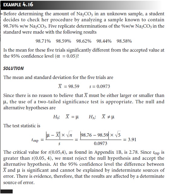
If evidence for a determinate error is found, as in Example 4.16, its source should be identified and corrected before analyzing additional samples. Failing to reject the null hypothesis, however, does not imply that the method is accurate, but only indicates that there is insufficient evidence to prove the method inaccurate at the stated confidence level.                          

The utility of the t-test for X– and μ is improved by optimizing the conditions used in determining X–. Examining equation 4.15 shows that increasing the num- ber of replicate determinations, n, or improving the precision of the analysis en- hances the utility of this significance test. A t-test can only give useful results, however, if the standard deviation for the analysis is reasonable. If the standard deviation is substantially larger than the expected standard deviation, σ, the confidence interval around X– will be so large that a significant difference between X– and μ may be difficult to prove. On the other hand, if the standard deviation is  significantly smaller than expected, the confidence interval around X will be too small, and a significant difference between X and μ may be found when none ex- ists. A significance test that can be used to evaluate the standard deviation is the subject of the next section.

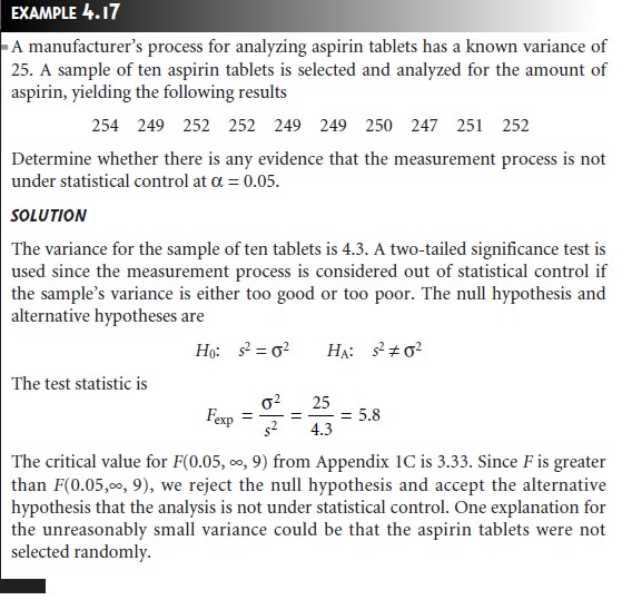
Comparing s2 to σ2

When a particular type of sample is analyzed on a regular basis, it may be possible to determine the expected, or true variance, σ 2, for the analysis. This often is the case in clinical labs where hundreds of blood samples are analyzed each day. Repli- cate analyses of any single sample, however, results in a sample variance, s2. A statis- tical comparison of s2 to σ2 provides useful information about whether the analysis is in a state of “statistical control.” The null hypothesis is that σ 2 and s2 are identical, and the alternative hypothesis is that they are not identical.

The test statistic for evaluating the null hypothesis is called an F-test, and is given as either

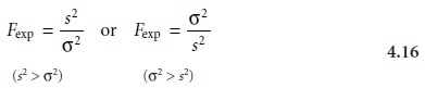
depending on whether s2 is larger or smaller than σ2. Note that F_exp is defined such that its value is always greater than or equal to 1.

If the null hypothesis is true, then F_exp should equal 1. Due to indeterminate er- rors, however, the value for F_exp usually is greater than 1. A critical value, F(α, v_num, v_den), gives the largest value of F that can be explained by indeterminate error. It is chosen for a specified significance level, α, and the degrees of freedom for the variances in the numerator, v_num, and denominator, v_den. The degrees of freedom for s2 is n – 1, where n is the number of replicates used in determining the sample’s vari- ance. Critical values of F for α = 0.05 are listed in Appendix 1C for both one-tailed and two-tailed significance tests.

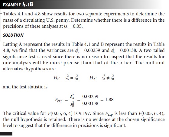
Comparing Two Sample Variances

The F-test can be extended to the comparison of variances for two samples, A and B, by rewriting equation 4.16 as

 where A and B are defined such that s²_A is greater than or equal to s²_B. An example of this application of the F-test is shown in the following example.

Comparing Two Sample Means

The result of an analysis is influenced by three factors: the method, the sample, and the analyst. The influence of these factors can be studied by conducting a pair of ex- periments in which only one factor is changed. For example, two methods can be compared by having the same analyst apply both methods to the same sample and examining the resulting means. In a similar fashion, it is possible to compare two analysts or two samples.

Significance testing for comparing two mean values is divided into two cate- gories depending on the source of the data. Data are said to be unpaired when each mean is derived from the analysis of several samples drawn from the same source. Paired data are encountered when analyzing a series of samples drawn from different sources.

Unpaired Data 

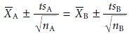
Consider two samples, A and B, for which mean values, X–_A, X–_B,, and standard deviations, s_A and s_B, have been measured. Confidence intervals for μ_A and μ_B can be written for both samples

where n_A and n_B are the number of replicate trials conducted on samples A and B. A comparison of the mean values is based on the null hypothesis that X–_A and X–_B are identical, and an alternative hypothesis that the means are significantly different.

A test statistic is derived by letting μ_A equal μ_B, and combining equations 4.17

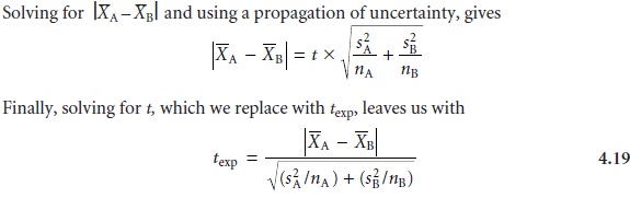
The value of t_exp is compared with a critical value, t(α, v), as determined by the cho- sen significance level, α, the degrees of freedom for the sample, v, and  whether the significance test is one-tailed or two-tailed.

It is unclear, however, how many degrees of freedom are associated with t(α, v) since there are two sets of independent measurements. If the variances s_A² and s_B² esti- mate the same σ2, then the two standard deviations can be factored out of equation 4.19 and replaced by a pooled standard deviation, s_pool, which provides a better esti- mate for the precision of the analysis. Thus, equation 4.19 becomes

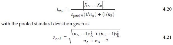
As indicated by the denominator of equation 4.21, the degrees of freedom for the pooled standard deviation is n_A + n_B – 2.

If s_A and s_B are significantly different, however, then t_exp must be calculated using equation 4.19. In this case, the degrees of freedom is calculated using the fol- lowing imposing equation.

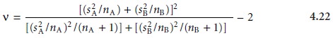
Since the degrees of freedom must be an integer, the value of v obtained using equation 4.22 is rounded to the nearest integer.

Regardless of whether equation 4.19 or 4.20 is used to calculate t_exp, the null hy- pothesis is rejected if t_exp is greater than t(α, v), and retained if t_exp is less than or equal to t(α, v).

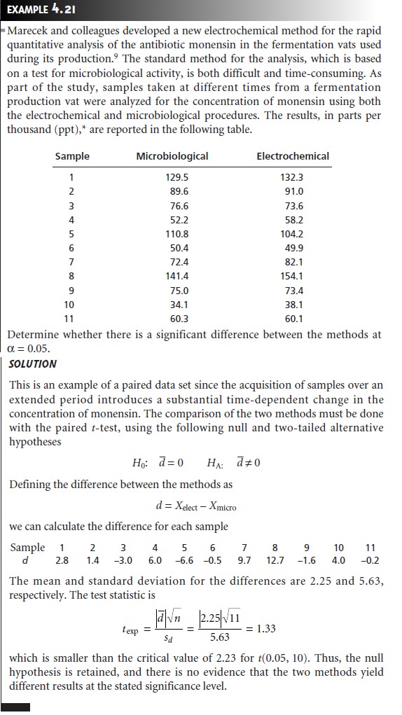
Paired Data 

In some situations the variation within the data sets being compared is more significant than the difference between the means of the two data sets. This is commonly encountered in clinical and environmental studies, where the data being compared usually consist of a set of samples drawn from several populations. For example, a study designed to investigate two procedures for monitoring the concentration of glucose in blood might involve blood samples drawn from ten pa- tients. If the variation in the blood glucose levels among the patients is significantly larger than the anticipated variation between the methods, then an analysis in which the data are treated as unpaired will fail to find a significant difference between the methods. In general, paired data sets are used whenever the variation being investi- gated is smaller than other potential sources of variation.

In a study involving paired data the difference, d , between the paired values for each sample is calculated. The average difference, d’, and standard deviation of the differences, s_d, are then calculated. The null hypothesis is that d is 0, and that there is no difference in the results for the two data sets. The alternative hypothesis is that the results for the two sets of data are significantly different, and, therefore, d is not equal to 0.                                              

The test statistic, t_exp, is derived from a confidence interval around d– 

where n is the number of paired samples. Replacing t with t_exp and rearranging gives

The value of t_exp is then compared with a critical value, t(α, v), which is determined by the chosen significance level, α, the degrees of freedom for the sample, v, and whether the significance test is one-tailed or two-tailed. For paired data, the degrees of freedom is n – 1. If t_exp is greater than t(α, v), then the null hypothesis is rejected and the alternative hypothesis is accepted. If t_exp is less than or equal to t(α, v), then the null hypothesis is retained, and a significant difference has not been demon- strated at the stated significance level. This is known as the paired t-test.

A paired t-test can only be applied when the individual differences, d_i, belong to the same population. This will only be true if the determinate and indeterminate errors affecting the results are independent of the concentration of analyte in the samples. If this is not the case, a single sample with a larger error could result in a value of d that is substantially larger than that for the remaining samples. Including this sample in the calculation of d– and s_d leads to a biased estimate of the true mean and standard deviation. For samples that span a limited range of analyte concentra- tions, such as that in Example 4.21, this is rarely a problem. When paired data span a wide range of concentrations, however, the magnitude of the determinate and in- determinate sources of error may not be independent of the analyte’s concentra- tion. In such cases the paired t-test may give misleading results since the paired data with the largest absolute determinate and indeterminate errors will dominate d–. In this situation a comparison is best made using a linear regression.

Outliers

On occasion, a data set appears to be skewed by the presence of one or more data points that are not consistent with the remaining data points. Such values are called outliers. The most commonly used significance test for identifying outliers is Dixon’s Q-test. The null hypothesis is that the apparent outlier is taken from the same popula- tion as the remaining data. The alternative hypothesis is that the outlier comes from a different population, and, therefore, should be excluded from consideration.

The Q-test compares the difference between the suspected outlier and its near- est numerical neighbor to the range of the entire data set. Data are ranked from smallest to largest so that the suspected outlier is either the first or the last data point. The test statistic, Q_exp, is calculated using equation 4.23 if the suspected out- lier is the smallest value (X₁)

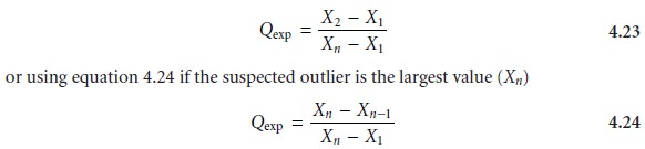
where n is the number of members in the data set, including the suspected outlier. It is important to note that equations 4.23 and 4.24 are valid only for the detection of a single outlier. Other forms of Dixon’s Q-test allow its extension to the detection of multiple outliers.10 The value of Q_exp is compared with a critical value, Q(α, n), at a significance level of α. The Q-test is usually applied as the more conservative two- tailed test, even though the outlier is the smallest or largest value in the data set. Values for Q(α, n) can be found in Appendix 1D. If Q_exp is greater than Q(α, n), then the null hypothesis is rejected and the outlier may be rejected. When Q_exp is less than or equal to Q(α, n) the suspected outlier must be retained.

The Q-test should be applied with caution since there is a probability, equal to α, that an outlier identified by the Q-test actually is not an outlier. In addition, the Q-test should be avoided when rejecting an outlier leads to a precision that is un- reasonably better than the expected precision determined by a propagation of un- certainty. Given these two concerns it is not surprising that some statisticians cau- tion against the removal of outliers. 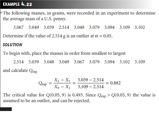On the other hand, testing for outliers can provide useful information if we try to understand the source of the suspected out- lier. For example, the outlier identified in Example 4.22 represents a significant change in the mass of a penny (an approximately 17% decrease in mass), due to a change in the composition of the U.S. penny. In 1982, the composition of a U.S. penny was changed from a brass alloy consisting of 95% w/w Cu and 5% w/w Zn, to a zinc core covered with copper. The pennies in Example 4.22 were therefore drawn from different populations.