Recursion

Recursion

Recursion is an algorithm design technique, closely related to induction. It is similar to iteration, but more powerful. Using recursion, we can solve a problem with a given input, by solving the instances of the problem with a part of the input.

Example 8.10. Customers are waiting in a line at a counter. The man at the counter wants to know how many customers are waiting in the line.

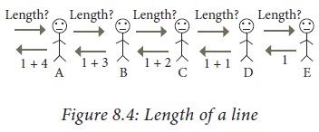
Instead of counting the length himself, he asks customer A for the length of the line with him at the head, customer A asks customer B for the length of the line with customer B at the head, and so on. When the query reaches the last customer in the line, E, since there is no one behind him, he replies 1 to D who asked him. D replies 1+1 = 2 to C, C replies 1+2 = 3 to B, B replies 1+3 = 4 to A, and A replies 1+4= 5 to the man in the counter

1. Recursive process

Example 8.10 illustrates a recursive process. Let us represent the sequence of 5 customers A, B, C, D and E as

[A,B,C,D,E]

The problem is to calculate the length of the sequence [A,B,C,D,E]. Let us name our solver length. If we pass a sequence as input, the solver length should output the length of the sequence.

length [A,B,C,D,E] = 5

Solver length breaks the sequence [A,B,C,D,E] into its first customer and the rest of the sequence.

first [A ,B,C,D,E] = A

rest [A ,B,C,D,E] = [B ,C,D,E]

To solve a problem recursively, solver length passes the reduced sequence [B,C,D,E] as input to a sub-solver, which is another instance of length. The solver assumes that the sub-solver outputs the length of [B,C,D,E], adds 1, and outputs it as the length of [A,B,C,D,E].

length [A,B,C,D,E] = 1 + length [B,C,D,E]

Each solver

1.           receives an input,

2.           passes an input of reduced size to a sub-solver,

3.           receives the solution to the reduced input from the sub-solver, and produces the solution for the given input as illustrated in Figure 8.5.

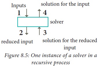
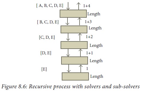
Figure 8.6 shows the input received and the solution produced by each solver for Example 8.10. Each solver reduces the size of the input by one and passes it on to a sub-solver, resulting in 5 solvers. This continues until the input received by a solver is small enough to output the solution directly. The last solver received [E] as the input. Since [E] is small enough, the solver outputs the length of [E] as 1 immediately, and the recursion stops.

The recursive process for length [A,B,C,D,E] is shown in Figure 8.7.

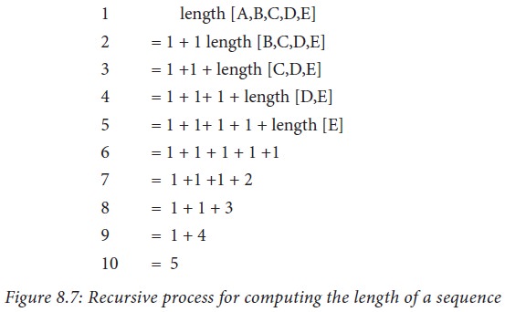
1 length [A,B,C,D,E]

2= 1 + 1 length [B,C,D,E]

3= 1 +1 + length [C,D,E]

4= 1 + 1+ 1 + length [D,E]

5= 1 + 1+ 1 + 1 + length [E]

6= 1 + 1 + 1 + 1 +1

7= 1 +1 +1 + 2

8= 1 + 1 + 3

9= 1 + 4

10 = 5

Figure 8.7: Recursive process for computing the length of a sequence

2. Recursive problem solving

Each solver should test the size of the input. If the size is small enough, the solver should output the solution to the problem directly. If the size is not small enough, the solver should reduce the size of the input and call a sub-solver to solve the problem with the reduced input. For Example 8.10, solver's algorithm can be expressed as length of sequesce.

To solve a problem recursively, the solver reduces the problem to sub-problems, and calls another instance of the solver, known as sub-solver, to solve the sub-problem. The input size to a sub-problem is smaller than the input size to the original problem. When the solver calls a sub-solver, it is known as recursive call. The magic of recursion allows the solver to assume that the sub-solver (recursive call) outputs the solution to the sub-problem. Then, from the solution to the sub-problem, the solver constructs the solution to the given problem.

As the sub-solvers go on reducing the problem into sub-problems of smaller sizes, eventually the sub-problem becomes small enough to be solved directly, without recursion. Therefore, a recursive solver has two cases:

1.           Base case: The problem size is small enough to be solved directly. Output the solution. There must be at least one base case.

2.           Recursion step: The problem size is not small enough. Deconstruct the problem into a sub-problem, strictly smaller in size than the given problem. Call a sub-solver to solve the sub-problem. Assume that the sub-solver outputs the solution to the sub-problem. Construct the solution to the given problem.

This outline of recursive problem solving technique is shown below.

solver (input)

if input is small enough

construct solution

else

find sub_problems of reduced

input

solutions to sub_problems =

solver for each sub_problem

construct solution to the 2 × 16

problem from

solutions to the sub_problems

Problems

Whenever we solve a problem using recursion, we have to ensure these two cases: In the recursion step, the size of the input to the recursive call is strictly smaller than the size of the given input, and there is at least one base case.

3. Recursion — Examples

Example 8.11. The recursive algorithm for length of a sequence can be written as

length (s)

--inputs : s

--outputs : length of s

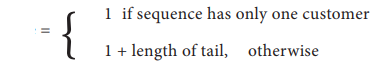
if s has one customer -- base case 1

else

1 + length(tail(s)) -- recursion step

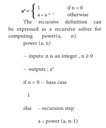
Example 8.12. Design a recursive algorithm to compute aⁿ. We constructed an iterative algorithm to compute aⁿ in Example 8.5. aⁿ can be defined recursively as

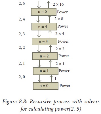
The recursive process with solvers for calculating power(2, 5) is shown in Figure 8.8.

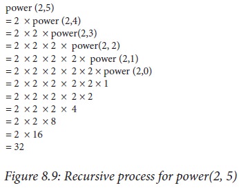
The recursive process resulting from power(2, 5) is shown in Figure 8.9.

power (2,5)

=2 × power (2,4)

=2 × 2 × power(2,3)

=2 × 2 × 2 × power(2, 2)

=2 × 2 × 2 × 2 × power (2,1)

=2 × 2 × 2 × 2 × 2 × power (2,0)

=2 × 2 × 2 × 2 × 2 × 1

=2 × 2 × 2 × 2 × 2

=2 × 2 × 2 × 4

=2 × 2 × 8

=2 × 16

=32

Figure 8.9: Recursive process for power(2, 5)

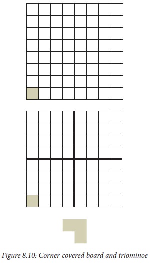
Example 8.13. A corner-covered board is a board of 2ⁿ × 2ⁿ squares in which the square at one corner is covered with a single square tile. A triominoe is a L-shaped tile formed with three adjacent squares (see Figure 8.10). Cover the corner-covered board with the L-shaped triominoes without overlap. Triominoes can be rotated as needed.

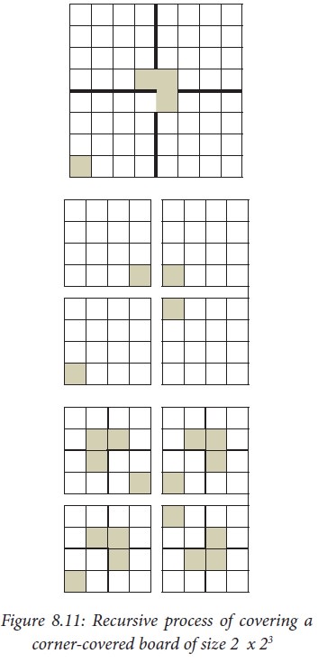
The size of the problem is n (board of size 2ⁿ × 2ⁿ). We can solve the problem by recursion. The base case is n = 1. It is a 2 × 2 corner-covered board. We can cover it with one triominoe and solve the problem. In the recursion step, divide the corner-covered board of size 2ⁿ × 2ⁿ into 4 sub-boards, each of size 2^n-1 × 2^n-1, by drawing horizontal and vertical lines through the centre of the board. Place atriominoe at the center of the entire board so as to not cover the corner-covered sub-board, as shown in the left-most board of Figure 8.11. Now, we have four corner-covered boards, each of size 2^n-1 × 2^n-1.

We have 4 sub-problems whose size is strictly smaller than the size of the given problem. We can solve each of the sub-problems recursively.

tile corner_covered board of size n

if n = 1 -- base case

cover  the  3  squares  with  one

triominoe

else -- recursion step

divide board into 4 sub_boards of size n-1

place a triominoe at centre of board ,

leaving out the corner_covered sub

-board

tile each sub_board of size n-1

The resulting recursive process for covering a 2³ x 2³ corner-covered board is illustrated in Figure 8.11.