Quicksort

Quicksort

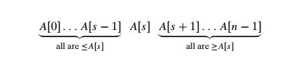
Quicksort is the other important sorting algorithm that is based on the divide-and-conquer approach. Unlike mergesort, which divides its input elements according to their position in the array, quicksort divides them according to their value. We already encountered this idea of an array partition in Section 4.5, where we discussed the selection problem. A partition is an arrangement of the array’s elements so that all the elements to the left of some element A[s] are less than or equal to A[s], and all the elements to the right of A[s] are greater than or equal to it:

Obviously, after a partition is achieved, A[s] will be in its final position in the sorted array, and we can continue sorting the two subarrays to the left and to the right of A[s] independently (e.g., by the same method). Note the difference with mergesort: there, the division of the problem into two subproblems is immediate and the entire work happens in combining their solutions; here, the entire work happens in the division stage, with no work required to combine the solutions to the subproblems.

Here is pseudocode of quicksort: call Quicksort(A[0..n − 1]) where

ALGORITHM                 Quicksort(A[l..r])

//Sorts a subarray by quicksort

//Input: Subarray of array A[0..n − 1], defined by its left and right

                        indices l and r

//Output: Subarray A[l..r] sorted in nondecreasing order

if l < r

s ←Partition(A[l..r]) //s is a split position

Quicksort(A[l..s − 1])

Quicksort(A[s + 1..r])

As a partition algorithm, we can certainly use the Lomuto partition discussed in Section 4.5. Alternatively, we can partition A[0..n − 1] and, more generally, its subarray A[l..r] (0 ≤ l < r ≤ n − 1) by the more sophisticated method suggested by C.A.R. Hoare, the prominent British computer scientist who invented quicksort.

As before, we start by selecting a pivot—an element with respect to whose value we are going to divide the subarray. There are several different strategies for selecting a pivot; we will return to this issue when we analyze the algorithm’s efficiency. For now, we use the simplest strategy of selecting the subarray’s first element: p = A[l].

Unlike the Lomuto algorithm, we will now scan the subarray from both ends, comparing the subarray’s elements to the pivot. The left-to-right scan, denoted below by index pointer i, starts with the second element. Since we want elements smaller than the pivot to be in the left part of the subarray, this scan skips over elements that are smaller than the pivot and stops upon encountering the first element greater than or equal to the pivot. The right-to-left scan, denoted below by index pointer j, starts with the last element of the subarray. Since we want elements larger than the pivot to be in the right part of the subarray, this scan skips over elements that are larger than the pivot and stops on encountering the first element smaller than or equal to the pivot. (Why is it worth stopping the scans after encountering an element equal to the pivot? Because doing this tends to yield more even splits for arrays with a lot of duplicates, which makes the algorithm run faster. For example, if we did otherwise for an array of n equal elements, we would have gotten a split into subarrays of sizes n − 1 and 0, reducing the problem size just by 1 after scanning the entire array.)

After both scans stop, three situations may arise, depending on whether or not the scanning indices have crossed. If scanning indices i and j have not crossed, i.e., i < j, we simply exchange A[i] and A[j ] and resume the scans by incrementing i and decrementing j, respectively:

ALGORITHM                 HoarePartition(A[l..r])

//Partitions a subarray by Hoare’s algorithm, using the first element

                        as a pivot

//Input: Subarray of array A[0..n − 1], defined by its left and right

                        indices l and r (l < r)

//Output: Partition of A[l..r], with the split position returned as

                        this function’s value

p ← A[l]

i ← l; j ← r + 1

repeat

repeat i ← i + 1 until A[i] ≥ p repeat j ← j − 1 until A[j ] ≤ p swap(A[i], A[j ])

until i ≥ j

swap(A[i], A[j ]) //undo last swap when i ≥ j swap(A[l], A[j ])

return j

Note that index i can go out of the subarray’s bounds in this pseudocode. Rather than checking for this possibility every time index i is incremented, we can append to array A[0..n − 1] a “sentinel” that would prevent index i from advancing beyond position n. Note that the more sophisticated method of pivot selection mentioned at the end of the section makes such a sentinel unnecessary.

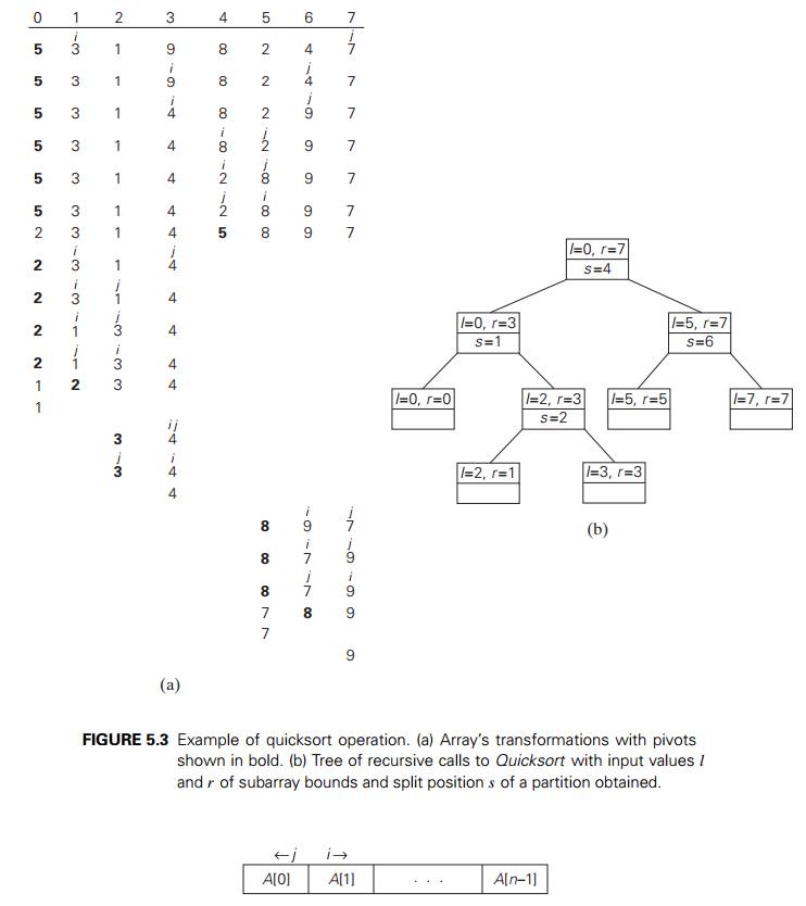
An example of sorting an array by quicksort is given in Figure 5.3.

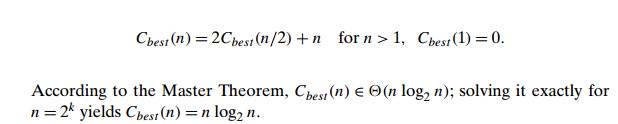
We start our discussion of quicksort’s efficiency by noting that the number of key comparisons made before a partition is achieved is n + 1 if the scanning indices cross over and n if they coincide (why?). If all the splits happen in the middle of corresponding subarrays, we will have the best case. The number of key comparisons in the best case satisfies the recurrence

In the worst case, all the splits will be skewed to the extreme: one of the two subarrays will be empty, and the size of the other will be just 1 less than the size of the subarray being partitioned. This unfortunate situation will happen, in particular, for increasing arrays, i.e., for inputs for which the problem is already solved! Indeed, if A[0..n − 1] is a strictly increasing array and we use A[0] as the pivot, the left-to-right scan will stop on A[1] while the right-to-left scan will go all the way to reach A[0], indicating the split at position 0:

So, after making n + 1 comparisons to get to this partition and exchanging the pivot A[0] with itself, the algorithm will be left with the strictly increasing array A[1..n − 1] to sort. This sorting of strictly increasing arrays of diminishing sizes will continue until the last one A[n − 2..n − 1] has been processed. The total number of key comparisons made will be equal to

Thus, the question about the utility of quicksort comes down to its average-case behavior. Let C_avg(n) be the average number of key comparisons made by quicksort on a randomly ordered array of size n. A partition can happen in any position s (0 ≤ s ≤ n − 1) after n + 1 comparisons are made to achieve the partition. After the partition, the left and right subarrays will have s and n − 1 − s elements, respectively. Assuming that the partition split can happen in each position s with the same probability 1/n, we get the following recurrence relation:

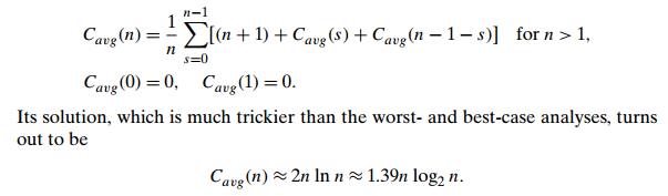
Thus, on the average, quicksort makes only 39% more comparisons than in the best case. Moreover, its innermost loop is so efficient that it usually runs faster than mergesort (and heapsort, another n log n algorithm that we discuss in Chapter 6) on randomly ordered arrays of nontrivial sizes. This certainly justifies the name given to the algorithm by its inventor.

Because of quicksort’s importance, there have been persistent efforts over the years to refine the basic algorithm. Among several improvements discovered by researchers are:

better pivot selection methods such as randomized quicksort that uses a random element or the median-of-three method that uses the median of the leftmost, rightmost, and the middle element of the array

switching to insertion sort on very small subarrays (between 5 and 15 elements for most computer systems) or not sorting small subarrays at all and finishing the algorithm with insertion sort applied to the entire nearly sorted array modifications of the partitioning algorithm such as the three-way partition into segments smaller than, equal to, and larger than the pivot (see Problem 9 in this section’s exercises)

According to Robert Sedgewick [Sed11, p. 296], the world’s leading expert on quicksort, such improvements in combination can cut the running time of the algorithm by 20%–30%.

Like any sorting algorithm, quicksort has weaknesses. It is not stable. It requires a stack to store parameters of subarrays that are yet to be sorted. While the size of this stack can be made to be in O(log n) by always sorting first the smaller of two subarrays obtained by partitioning, it is worse than the O(1) space efficiency of heapsort. Although more sophisticated ways of choosing a pivot make the quadratic running time of the worst case very unlikely, they do not eliminate it completely. And even the performance on randomly ordered arrays is known to be sensitive not only to implementation details of the algorithm but also to both computer architecture and data type. Still, the January/February 2000 issue of Computing in Science & Engineering, a joint publication of the American Institute of Physics and the IEEE Computer Society, selected quicksort as one of the 10 algorithms “with the greatest influence on the development and practice of science and engineering in the 20th century.”

Exercises 5.2

         1. Apply quicksort to sort the list E, X, A, M, P , L, E in alphabetical order. Draw the tree of the recursive calls made.

2. For the partitioning procedure outlined in this section:

         Prove that if the scanning indices stop while pointing to the same element, i.e., i = j, the value they are pointing to must be equal to p.

         Prove that when the scanning indices stop, j cannot point to an element more than one position to the left of the one pointed to by i.

         Give an example showing that quicksort is not a stable sorting algorithm.

         Give an example of an array of n elements for which the sentinel mentioned in the text is actually needed. What should be its value? Also explain why a single sentinel suffices for any input.

         For the version of quicksort given in this section:

         Are arrays made up of all equal elements the worst-case input, the best-case input, or neither?

         Are strictly decreasing arrays the worst-case input, the best-case input, or neither?

                 a. For quicksort with the median-of-three pivot selection, are strictly increas-ing arrays the worst-case input, the best-case input, or neither?

         Answer the same question for strictly decreasing arrays.

                 a. Estimate how many times faster quicksort will sort an array of one million random numbers than insertion sort.

         True or false: For every n > 1, there are n-element arrays that are sorted faster by insertion sort than by quicksort?

Design an algorithm to rearrange elements of a given array of n real num-bers so that all its negative elements precede all its positive elements. Your algorithm should be both time efficient and space efficient.

                 a. The Dutch national flag problem is to rearrange an array of characters R, W , and B (red, white, and blue are the colors of the Dutch national flag) so that all the R’s come first, the W ’s come next, and the B’s come last. [Dij76] Design a linear in-place algorithm for this problem.

         Explain how a solution to the Dutch national flag problem can be used in quicksort.

            Implement quicksort in the language of your choice. Run your program on a sample of inputs to verify the theoretical assertions about the algorithm’s efficiency.

11. Nuts and bolts You are given a collection of n bolts of different widths and n corresponding nuts. You are allowed to try a nut and bolt together, from which you can determine whether the nut is larger than the bolt, smaller than the bolt, or matches the bolt exactly. However, there is no way to compare two nuts together or two bolts together. The problem is to match each bolt to its nut. Design an algorithm for this problem with average-case efficiency in  ѳ(n log n). [Raw91]