Problem of Dimensionality- Dynamic Programming

PROBLEM OF DIMENSIONALITY

In all the DP models we presented, the state at any stage is represented by a single element. For example, in the knapsack model (Section 10.3.1), the only restriction is the weight of the item. More realistically, the volume of the knapsack may also be another viable restriction. In such a case, the state at any stage is said to be two-dimensional because it consists of two elements: weight and volume.

The increase in the number of state variables increases the computations at each stage. This is particularly clear in DP tabular computations because the number of rows in each tableau corresponds to all possible combinations of state variables.

This computational difficulty is sometimes referred to in the literature as the curse of dimensionality.

The following example is chosen to demonstrate the problem of dimensionality. It also serves to show the relationship between linear and dynamic programming.

Example 10.4-1

Acme Manufacturing produces two products. The daily capacity of the manufacturing process is 430 minutes. Product 1 requires 2 minutes per unit, and product 2 requires 1 minute per unit. There is no limit on the amount produced of product 1, but the maximum daily demand for product 2 is 230 units. The unit profit of product 1 is $2 and that of product 2 is $5. Find the optimal solution by DP.

The problem is represented by the following linear program:

The elements of the DP model are

1.  Stage i corresponds to product i, i = 1, 2.

2.  Alternative x_i is the amount of product i, i =  1,2.

3.  State (v₂, w₂) represents the amounts of resources 1 and 2 (production time and demand limits) used in stage 2.

4.  State (v₁, w₁) represents the amounts of resources 1 and 2 (production time and demand limits) used in stages 1 and 2.

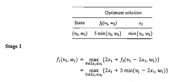
Stage 2. Define f₂(v₂,w₂) as the maximum profit for stage 2 (product 2), given the state (v₂,w₂). Then .

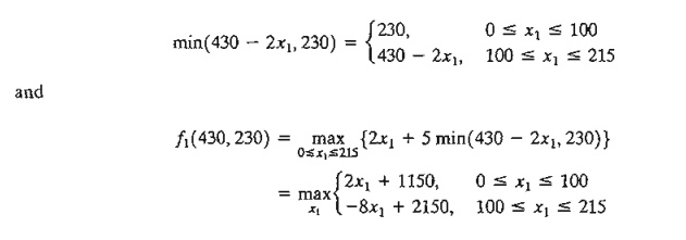
The optimization of stage 1 requires the solution of a (generally difficult) minimax problem. For the present problem, we set v₁ = 430 and w₁ = 230, which gives 0 ≤ 2x₁ ≤  430. Because mine (430 – 2x_i, 230) is the lower envelope of two intersecting lines (verify!), it follows that

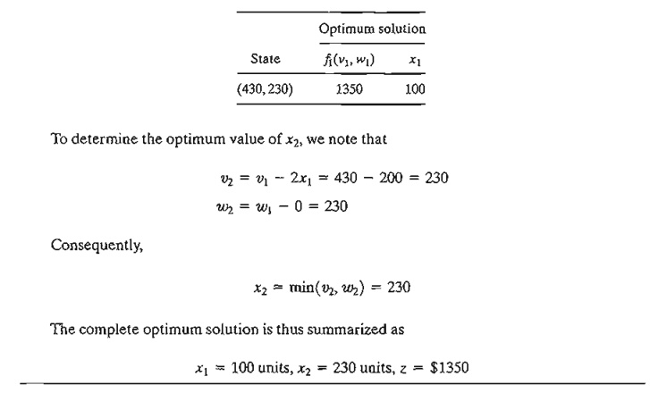
You can verify graphically that the optimum value of f₁ (430,230) occurs at x₁ = 100. Thus, we get

2. In the n-item knapsack problem of Example 10.3-1, suppose that the weight and volume limitations are Wand V, respectively. Given that w_i, v_j, and rj are the weight, value, and revenue per unit of item i, write the DP backward recursive equation for the problem.