Chapter: Operations Research: An Introduction : Deterministic Dynamic Programming
Forward and Backward Recursion- Dynamic Programming
FORWARD AND BACKWARD RECURSION
Example 10.1-1 uses forward recursion in which the computations
proceed from stage 1 to stage 3. The same example can be solved by backward recursion, starting at stage 3 and ending at stage l.
Both the forward and backward recursions yield the same solution.
Although the forward procedure appears more logical, DP literature invariably
uses backward recursion. The reason for this preference is that, in general,
backward recursion may be more efficient computationally. We will demonstrate
the use of backward recursion by applying it to Example 10.1-1. The
demonstration will also provide the opportunity to present the DP computations
in a compact tabular form.
Example 10.2-1
The
backward recursive equation for Example 10.2-1 is
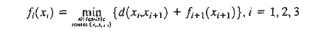
where f4(x4) = 0 for x4 = 7. The associated order of computations is f3 - > f2- >f1.
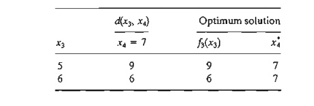
Stage 3. Because node 7 (x4 = 7) is connected to
nodes 5 and 6 (x3 = 5 and
6) with exactly one route each, there are no alternatives to choose from, and
stage 3 results can be summarized as
Stage 2. Route (2, 6) is blocked because
it does not exist. Given f3(x3)
from stage 3, we can compare the feasible alternatives as shown in the
following tableau:
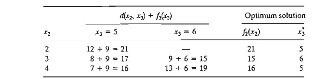
The
optimum solution of stage 2 reads as follows: If you are in cities 2 or 4, the shortest route passes through city 5, and
if you are in city 3, the shortest route passes through city 6.
Stage 1.
From node 1, we have three alternative routes: (1,2), (1, 3), and (1,4). Using h(X2) from
stage 2. we can compute the following tableau.
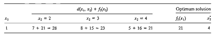
The
optimum solution at stage 1 shows that city 1 is linked to city 4. Next, the
optimum solution at stage 2 links city 4 to city 5. Finally. the optimum
solution at stage 3 connects city 5 to city 7. Thus, the complete route is
given as 1 -> 4 -> 5 -> 7. and the
associated distance is 21 miles.
PROBLEM SET 10.2A
For
Problem 1, Set 10.1a, develop the backward recursive equation, and use it to find
the optimum solution.
2. For Problem 2, Set l0..la, develop the backward recursive equation,
and use it to find the optimum solution.
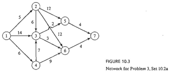
*3. For the network in Figure 10.3, it is desired to determine the
shortest route between cities 1 to 7. Define the stages and the states using
backward recursion, and then solve the problem.
Related Topics