Parallel Hardware

PARALLEL HARDWARE

Multiple issue and pipelining can clearly be considered to be parallel hardware, since functional units are replicated. However, since this form of parallelism isn’t usually visible to the programmer, we’re treating both of them as extensions to the basic von Neumann model, and for our purposes, parallel hardware will be limited to hardware that’s visible to the programmer. In other words, if she can readily modify her source code to exploit it, or if she must modify her source code to exploit it, then we’ll consider the hardware to be parallel.

1. SIMD systems

In parallel computing, Flynn’s taxonomy  is frequently used to classify computer architectures. It classifies a system according to the number of instruction streams and the number of data streams it can simultaneously manage. A classical von Neumann system is therefore a single instruction stream, single data stream, or SISD system, since it executes a single instruction at a time and it can fetch or store one item of data at a time.

Single instruction, multiple data, or SIMD, systems are parallel systems. As the name suggests, SIMD systems operate on multiple data streams by applying the same instruction to multiple data items, so an abstract SIMD system can be thought of as having a single control unit and multiple ALUs. An instruction is broadcast from the control unit to the ALUs, and each ALU either applies the instruction to the current data item, or it is idle. As an example, suppose we want to carry out a “vector addition.” That is, suppose we have two arrays x and y, each with n elements, and we want to add the elements of y to the elements of x:

for (i = 0; i < n; i++)

x[i] += y[i];

Suppose further that our SIMD system has n ALUs. Then we could load x[i] and y[i] into the ith ALU, have the ith ALU add y[i] to x[i], and store the result in x[i]. If the system has m ALUs and m < n, we can simply execute the additions in blocks of m elements at a time. For example, if m D 4 and n D 15, we can first add ele-ments 0 to 3, then elements 4 to 7, then elements 8 to 11, and finally elements 12 to 14. Note that in the last group of elements in our example—elements 12 to 14—we’re only operating on three elements of x and y, so one of the four ALUs will be idle.

The requirement that all the ALUs execute the same instruction or are idle can seriously degrade the overall performance of a SIMD system. For example, suppose we only want to carry out the addition if y[i] is positive:

for (i = 0; i < n; i++)

if (y[i] > 0.0) x[i] += y[i];

In this setting, we must load each element of y into an ALU and determine whether it’s positive. If y[i] is positive, we can proceed to carry out the addition. Otherwise, the ALU storing y[i] will be idle while the other ALUs carry out the addition.

Note also that in a “classical” SIMD system, the ALUs must operate syn-chronously, that is, each ALU must wait for the next instruction to be broadcast before proceeding. Further, the ALUs have no instruction storage, so an ALU can’t delay execution of an instruction by storing it for later execution.

Finally, as our first example shows, SIMD systems are ideal for parallelizing sim-ple loops that operate on large arrays of data. Parallelism that’s obtained by dividing data among the processors and having the processors all apply (more or less) the same instructions to their subsets of the data is called data-parallelism. SIMD parallelism can be very efficient on large data parallel problems, but SIMD systems often don’t do very well on other types of parallel problems.

SIMD systems have had a somewhat checkered history. In the early 1990s a maker of SIMD systems (Thinking Machines) was the largest manufacturer of par-allel supercomputers. However, by the late 1990s the only widely produced SIMD systems were vector processors. More recently, graphics processing units, or GPUs, and desktop CPUs are making use of aspects of SIMD computing.

Vector processors

Although what constitutes a vector processor has changed over the years, their key characteristic is that they can operate on arrays or vectors of data, while conventional CPUs operate on individual data elements or scalars. Typical recent systems have the following characteristics:

Vector registers. These are registers capable of storing a vector of operands and operating simultaneously on their contents. The vector length is fixed by the

system, and can range from 4 to 128 64-bit elements.

Vectorized and pipelined functional units. Note that the same operation is applied

to each element in the vector, or, in the case of operations like addition, the same operation is applied to each pair of corresponding elements in the two vectors.

Thus, vector operations are SIMD.

Vector instructions. These are instructions that operate on vectors rather than scalars. If the vector length is vector length, these instructions have the great virtue that a simple loop such as

for (i = 0; i < n; i++)

x[i] += y[i];

requires only a single load, add, and store for each block of vector length elements, while a conventional system requires a load, add, and store for each

^element.Interleaved memory. The memory system consists of multiple “banks” of memory, which can be accessed more or less independently. After accessing one bank, there will be a delay before it can be reaccessed, but a different bank can be accessed

much sooner. So if the elements of a vector are distributed across multiple banks,

there can be little to no delay in loading/storing successive elements.

Strided memory access and hardware scatter/gather. In strided memory access, the program accesses elements of a vector located at fixed intervals. For example, accessing the first element, the fifth element, the ninth element, and so on, would be strided access with a stride of four. Scatter/gather (in this context) is writing (scatter) or reading (gather) elements of a vector located at irregular intervals— for example, accessing the first element, the second element, the fourth element, the eighth element, and so on. Typical vector systems provide special hardware to accelerate strided access and scatter/gather.

Vector processors have the virtue that for many applications, they are very fast and very easy to use. Vectorizing compilers are quite good at identifying code that can be vectorized. Further, they identify loops that cannot be vectorized, and they often provide information about why a loop couldn’t be vectorized. The user can thereby make informed decisions about whether it’s possible to rewrite the loop so that it will vectorize. Vector systems have very high memory bandwidth, and every data item that’s loaded is actually used, unlike cache-based systems that may not make use of every item in a cache line. On the other hand, they don’t handle irregular data struc-tures as well as other parallel architectures, and there seems to be a very finite limit to their scalability, that is, their ability to handle ever larger problems. It’s difficult to see how systems could be created that would operate on ever longer vectors. Cur-rent generation systems scale by increasing the number of vector processors, not the vector length. Current commodity systems provide limited support for operations on very short vectors, while processors that operate on long vectors are custom manufactured, and, consequently, very expensive.

Graphics processing units

Real-time graphics application programming interfaces, or APIs, use points, lines, and triangles to internally represent the surface of an object. They use a graphics pro-cessing pipeline to convert the internal representation into an array of pixels that can

be sent to a computer screen. Several of the stages of this pipeline are programmable. The behavior of the programmable stages is specified by functions called shader functions. The shader functions are typically quite short—often just a few lines of C code. They’re also implicitly parallel, since they can be applied to multiple elements (e.g., vertices) in the graphics stream. Since the application of a shader function to nearby elements often results in the same flow of control, GPUs can optimize perfor-mance by using SIMD parallelism, and in the current generation all GPUs use SIMD parallelism. This is obtained by including a large number of ALUs (e.g., 80) on each GPU processing core.

Processing a single image can require very large amounts of data—hundreds of megabytes of data for a single image is not unusual. GPUs therefore need to maintain very high rates of data movement, and in order to avoid stalls on memory accesses, they rely heavily on hardware multithreading; some systems are capable of storing the state of more than a hundred suspended threads for each executing thread. The actual number of threads depends on the amount of resources (e.g., registers) needed by the shader function. A drawback here is that many threads processing a lot of data are needed to keep the ALUs busy, and GPUs may have relatively poor performance on small problems.

It should be stressed that GPUs are not pure SIMD systems. Although the ALUs on a given core do use SIMD parallelism, current generation GPUs can have dozens of cores, which are capable of executing independent instruction streams.

GPUs are becoming increasingly popular for general, high-performance comput-ing, and several languages have been developed that allow users to exploit their power. For further details see [30].

2. MIMD systems

Multiple instruction, multiple data, or MIMD, systems support multiple simulta-neous instruction streams operating on multiple data streams. Thus, MIMD systems typically consist of a collection of fully independent processing units or cores, each of which has its own control unit and its own ALU. Furthermore, unlike SIMD sys-tems, MIMD systems are usually asynchronous, that is, the processors can operate at their own pace. In many MIMD systems there is no global clock, and there may be no relation between the system times on two different processors. In fact, unless the programmer imposes some synchronization, even if the processors are executing exactly the same sequence of instructions, at any given instant they may be executing different statements.

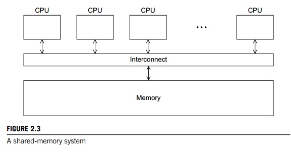
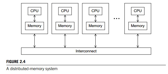
As we noted in Chapter 1, there are two principal types of MIMD systems: shared-memory systems and distributed-memory systems. In a shared-memory sys-tem a collection of autonomous processors is connected to a memory system via an interconnection network, and each processor can access each memory location. In a shared-memory system, the processors usually communicate implicitly by accessing shared data structures. In a distributed-memory system, each processor is paired with its own private memory, and the processor-memory pairs communicate over an interconnection network. So in distributed-memory systems the processors usu-ally communicate explicitly by sending messages or by using special functions that provide access to the memory of another processor. See Figures 2.3 and 2.4.

Shared-memory systems

The most widely available shared-memory systems use one or more multicore pro-cessors. As we discussed in Chapter 1, a multicore processor has multiple CPUs or cores on a single chip. Typically, the cores have private level 1 caches, while other caches may or may not be shared between the cores.

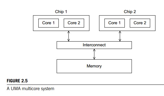
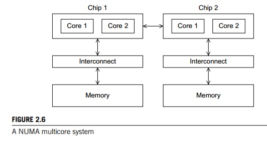
In shared-memory systems with multiple multicore processors, the interconnect can either connect all the processors directly to main memory or each processor can have a direct connection to a block of main memory, and the processors can access each others’ blocks of main memory through special hardware built into the pro-cessors. See Figures 2.5 and 2.6. In the first type of system, the time to access all the memory locations will be the same for all the cores, while in the second type a memory location to which a core is directly connected can be accessed more quickly than a memory location that must be accessed through another chip. Thus, the first type of system is called a uniform memory access, or UMA, system, while the sec-ond type is called a nonuniform memory access, or NUMA, system. UMA systems are usually easier to program, since the programmer doesn’t need to worry about different access times for different memory locations. This advantage can be offset by the faster access to the directly connected memory in NUMA systems. Further-more, NUMA systems have the potential to use larger amounts of memory than UMA systems.

Distributed-memory systems

The most widely available distributed-memory systems are called clusters. They are composed of a collection of commodity systems—for example, PCs—connected by a commodity interconnection network—for example, Ethernet. In fact, the nodes of these systems, the individual computational units joined together by the commu-nication network, are usually shared-memory systems with one or more multicore processors. To distinguish such systems from pure distributed-memory systems, they are sometimes called hybrid systems. Nowadays, it’s usually understood that a cluster will have shared-memory nodes.

The grid provides the infrastructure necessary to turn large networks of geograph-ically distributed computers into a unified distributed-memory system. In general, such a system will be heterogeneous, that is, the individual nodes may be built from different types of hardware.

3. Interconnection networks

The interconnect plays a decisive role in the performance of both distributed- and shared-memory systems: even if the processors and memory have virtually unlimited performance, a slow interconnect will seriously degrade the overall performance of all but the simplest parallel program. See, for example, Exercise 2.10.

Although some of the interconnects have a great deal in common, there are enough differences to make it worthwhile to treat interconnects for shared-memory and distributed-memory separately.

Shared-memory interconnects

Currently the two most widely used interconnects on shared-memory systems are buses and crossbars. Recall that a bus is a collection of parallel communication wires together with some hardware that controls access to the bus. The key characteristic of a bus is that the communication wires are shared by the devices that are connected to it. Buses have the virtue of low cost and flexibility; multiple devices can be con-nected to a bus with little additional cost. However, since the communication wires are shared, as the number of devices connected to the bus increases, the likelihood that there will be contention for use of the bus increases, and the expected perfor-mance of the bus decreases. Therefore, if we connect a large number of processors to a bus, we would expect that the processors would frequently have to wait for access to main memory. Thus, as the size of shared-memory systems increases, buses are rapidly being replaced by switched interconnects.

As the name suggests, switched interconnects use switches to control the rout-ing of data among the connected devices. A crossbar is illustrated in Figure 2.7(a). The lines are bidirectional communication links, the squares are cores or memory modules, and the circles are switches.

The individual switches can assume one of the two configurations shown in Figure 2.7(b). With these switches and at least as many memory modules as pro-cessors, there will only be a conflict between two cores attempting to access memory

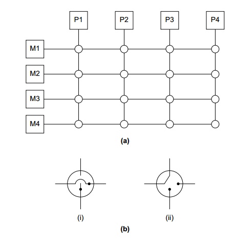
if the two cores attempt to simultaneously access the same memory module. For example, Figure 2.7(c) shows the configuration of the switches if P₁ writes to M₄, P₂ reads from M₃, P₃ reads from M₁, and P₄ writes to M₂.

Crossbars allow simultaneous communication among different devices, so they are much faster than buses. However, the cost of the switches and links is relatively high. A small bus-based system will be much less expensive than a crossbar-based system of the same size.

Distributed-memory interconnects

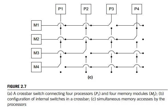
Distributed-memory interconnects are often divided into two groups: direct inter-connects and indirect interconnects. In a direct interconnect each switch is directly connected to a processor-memory pair, and the switches are connected to each other. Figure 2.8 shows a ring and a two-dimensional toroidal mesh. As before, the circles are switches, the squares are processors, and the lines are bidirectional links. A ring is superior to a simple bus since it allows multiple simultaneous communications. However, it’s easy to devise communication schemes in which some of the processors must wait for other processors to complete their communications. The toroidal mesh will be more expensive than the ring, because the switches are more complex—they must support five links instead of three—and if there are p processors, the number of links is 3p in a toroidal mesh, while it’s only 2p in a ring. However, it’s not difficult to convince yourself that the number of possible simultaneous communications patterns is greater with a mesh than with a ring.

One measure of “number of simultaneous communications” or “connectivity” is bisection width. To understand this measure, imagine that the parallel system is

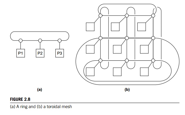
divided into two halves, and each half contains half of the processors or nodes. How many simultaneous communications can take place “across the divide” between the halves? In Figure 2.9(a) we’ve divided a ring with eight nodes into two groups of four nodes, and we can see that only two communications can take place between the halves. (To make the diagrams easier to read, we’ve grouped each node with its switch in this and subsequent diagrams of direct interconnects.) However, in Figure 2.9(b) we’ve divided the nodes into two parts so that four simultaneous com-munications can take place, so what’s the bisection width? The bisection width is supposed to give a “worst-case” estimate, so the bisection width is two—not four.

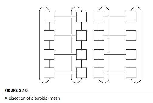
An alternative way of computing the bisection width is to remove the minimum number of links needed to split the set of nodes into two equal halves. The number of links removed is the bisection width. If we have a square two-dimensional toroidal mesh with p = q² nodes (where q is even), then we can split the nodes into two halves by removing the “middle” horizontal links and the “wraparound” horizontal links. See Figure 2.10. This suggests that the bisection width is at most 2q = 2^Rootp. In fact, this is the smallest possible number of links and the bisection width of a square two-dimensional toroidal mesh is 2^Rootp.

The bandwidth of a link is the rate at which it can transmit data. It’s usually given in megabits or megabytes per second. Bisection bandwidth is often used as a measure of network quality. It’s similar to bisection width. However, instead of counting the number of links joining the halves, it sums the bandwidth of the links. For example, if the links in a ring have a bandwidth of one billion bits per second, then the bisection bandwidth of the ring will be two billion bits per second or 2000 megabits per second.

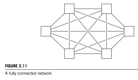
The ideal direct interconnect is a fully connected network in which each switch is directly connected to every other switch. See Figure 2.11. Its bisection width is p²=4. However, it’s impractical to construct such an interconnect for systems with more than a few nodes, since it requires a total of p²=2 + p=2 links, and each switch must be capable of connecting to p links. It is therefore more a “theoretical best possible” interconnect than a practical one, and it is used as a basis for evaluating other interconnects.

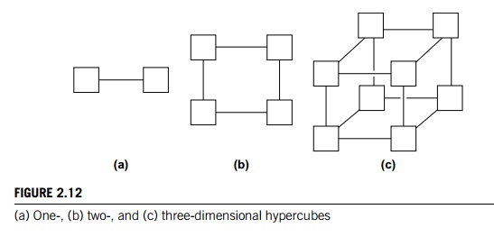
The hypercube is a highly connected direct interconnect that has been used in actual systems. Hypercubes are built inductively: A one-dimensional hypercube is a fully-connected system with two processors. A two-dimensional hypercube is built from two one-dimensional hypercubes by joining “corresponding” switches. Simi-larly, a three-dimensional hypercube is built from two two-dimensional hypercubes. See Figure 2.12. Thus, a hypercube of dimension d has p = 2^d nodes, and a switch in a d-dimensional hypercube is directly connected to a processor and d switches. The bisection width of a hypercube is p=2, so it has more connectivity than a ring or toroidal mesh, but the switches must be more powerful, since they must support 1 + d = 1 + log₂.p/ wires, while the mesh switches only require five wires. So a hypercube with p nodes is more expensive to construct than a toroidal mesh.

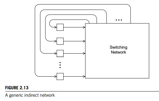
Indirect interconnects provide an alternative to direct interconnects. In an indi-rect interconnect, the switches may not be directly connected to a processor. They’re often shown with unidirectional links and a collection of processors, each of which has an outgoing and an incoming link, and a switching network. See Figure 2.13.

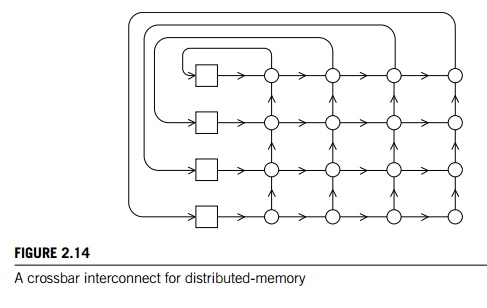
The crossbar and the omega network are relatively simple examples of indi-rect networks. We saw a shared-memory crossbar with bidirectional links earlier (Figure 2.7). The diagram of a distributed-memory crossbar in Figure 2.14 has unidi-rectional links. Notice that as long as two processors don’t attempt to communicate with the same processor, all the processors can simultaneously communicate with another processor.

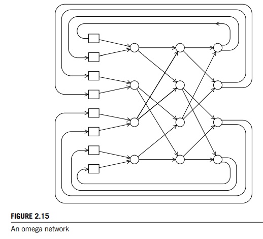
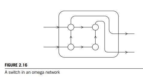
An omega network is shown in Figure 2.15. The switches are two-by-two cross-bars (see Figure 2.16). Observe that unlike the crossbar, there are communications that cannot occur simultaneously. For example, in Figure 2.15 if processor 0 sends

a message to processor 6, then processor 1 cannot simultaneously send a message to processor 7. On the other hand, the omega network is less expensive than the crossbar. The omega network uses ¹₂ p log₂(p) of the 2 2 crossbar switches, so it uses a total of 2p log₂(p) switches, while the crossbar uses p².

It’s a little bit more complicated to define bisection width for indirect networks. See Exercise 2.14. However, the principle is the same: we want to divide the nodes into two groups of equal size and determine how much communication can take place between the two halves, or alternatively, the minimum number of links that need to be removed so that the two groups can’t communicate. The bisection width of a p p crossbar is p and the bisection width of an omega network is p=2.

Latency and bandwidth

Any time data is transmitted, we’re interested in how long it will take for the data to reach its destination. This is true whether we’re talking about transmitting data between main memory and cache, cache and register, hard disk and memory, or between two nodes in a distributed-memory or hybrid system. There are two figures that are often used to describe the performance of an interconnect (regardless of what it’s connecting): the latency and the bandwidth. The latency is the time that elapses between the source’s beginning to transmit the data and the destination’s starting to receive the first byte. The bandwidth is the rate at which the destination receives data after it has started to receive the first byte. So if the latency of an interconnect is l seconds and the bandwidth is b bytes per second, then the time it takes to transmit a message of n bytes is

message transmission time = l + n=b.

Beware, however, that these terms are often used in different ways. For example, latency is sometimes used to describe total message transmission time. It’s also often used to describe the time required for any fixed overhead involved in transmitting data. For example, if we’re sending a message between two nodes in a distributed-memory system, a message is not just raw data. It might include the data to be transmitted, a destination address, some information specifying the size of the mes-sage, some information for error correction, and so on. So in this setting, latency might be the time it takes to assemble the message on the sending side—the time needed to combine the various parts—and the time to disassemble the message on the receiving side—the time needed to extract the raw data from the message and store it in its destination.

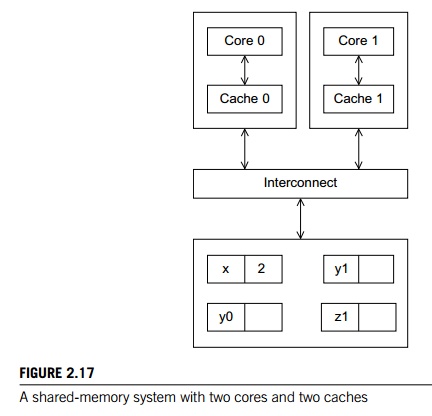
4. Cache coherence

Recall that CPU caches are managed by system hardware: programmers don’t have direct control over them. This has several important consequences for shared-memory systems. To understand these issues, suppose we have a shared-memory system with two cores, each of which has its own private data cache. See Figure 2.17. As long as the two cores only read shared data, there is no problem. For example, suppose that x is a shared variable that has been initialized to 2, y0 is private and owned by core 0, and y1 and z1 are private and owned by core 1. Now suppose the following statements are executed at the indicated times:

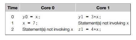
Then the memory location for y0 will eventually get the value 2, and the memory location for y1 will eventually get the value 6. However, it’s not so clear what value z1 will get. It might at first appear that since core 0 updates x to 7 before the assign-ment to z1, z1 will get the value 4 7 = 28. However, at time 0, x is in the cache of core 1. So unless for some reason x is evicted from core 0’s cache and then reloaded into core 1’s cache, it actually appears that the original value x = 2 may be used, and z1 will get the value 4 2 = 8.

Note that this unpredictable behavior will occur regardless of whether the system is using a write-through or a write-back policy. If it’s using a write-through policy, the main memory will be updated by the assignment x = 7. However, this will have no effect on the value in the cache of core 1. If the system is using a write-back policy, the new value of x in the cache of core 0 probably won’t even be available to core 1 when it updates z1.

Clearly, this is a problem. The programmer doesn’t have direct control over when the caches are updated, so her program cannot execute these apparently innocu-ous statements and know what will be stored in z1. There are several problems here, but the one we want to look at right now is that the caches we described for single processor systems provide no mechanism for insuring that when the caches of multiple processors store the same variable, an update by one processor to the cached variable is “seen” by the other processors. That is, that the cached value stored by the other processors is also updated. This is called the cache coherence problem.

Snooping cache coherence

There are two main approaches to insuring cache coherence: snooping cache coher-ence and directory-based cache coherence. The idea behind snooping comes from bus-based systems: When the cores share a bus, any signal transmitted on the bus can be “seen” by all the cores connected to the bus. Thus, when core 0 updates the copy of x stored in its cache, if it also broadcasts this information across the bus, and if core 1 is “snooping” the bus, it will see that x has been updated and it can mark its copy of x as invalid. This is more or less how snooping cache coherence works. The principal difference between our description and the actual snooping protocol is that the broadcast only informs the other cores that the cache line containing x has been updated, not that x has been updated.

A couple of points should be made regarding snooping. First, it’s not essential that the interconnect be a bus, only that it support broadcasts from each processor to all the other processors. Second, snooping works with both write-through and write-back caches. In principle, if the interconnect is shared—as with a bus—with write-through caches there’s no need for additional traffic on the interconnect, since each core can simply “watch” for writes. With write-back caches, on the other hand, an extra communication is necessary, since updates to the cache don’t get immediately sent to memory.

Directory-based cache coherence

Unfortunately, in large networks broadcasts are expensive, and snooping cache coher-ence requires a broadcast every time a variable is updated (but see Exercise 2.15). So snooping cache coherence isn’t scalable, because for larger systems it will cause performance to degrade. For example, suppose we have a system with the basic distributed-memory architecture (Figure 2.4). However, the system provides a single address space for all the memories. So, for example, core 0 can access the vari-able x stored in core 1’s memory, by simply executing a statement such as y = x.

(Of course, accessing the memory attached to another core will be slower than access-ing “local” memory, but that’s another story.) Such a system can, in principle, scale to very large numbers of cores. However, snooping cache coherence is clearly a problem since a broadcast across the interconnect will be very slow relative to the speed of accessing local memory.

Directory-based cache coherence protocols attempt to solve this problem through the use of a data structure called a directory. The directory stores the status of each cache line. Typically, this data structure is distributed; in our example, each core/memory pair might be responsible for storing the part of the structure that spec-ifies the status of the cache lines in its local memory. Thus, when a line is read into, say, core 0’s cache, the directory entry corresponding to that line would be updated indicating that core 0 has a copy of the line. When a variable is updated, the directory is consulted, and the cache controllers of the cores that have that variable’s cache line in their caches are invalidated.

Clearly there will be substantial additional storage required for the directory, but when a cache variable is updated, only the cores storing that variable need to be contacted.

False sharing

It’s important to remember that CPU caches are implemented in hardware, so they operate on cache lines, not individual variables. This can have disastrous conse-quences for performance. As an example, suppose we want to repeatedly call a function f(i,j) and add the computed values into a vector:

int i, j, m, n; double  y[m];

/*                      Assign y = 0       */

. . .

for (i = 0; i < m; i++) for (j = 0; j < n; j++)

y[i] += f(i,j);

We can parallelize this by dividing the iterations in the outer loop among the cores. If we have core count cores, we might assign the first m/core count iterations to the first core, the next m/core count iterations to the second core, and so on.

/* Private variables */

int i, j, iter count;

/ Shared variables initialized by one core */

int m, n, core count

double y[m];

iter count = m/core count

/*  Core 0 does this */

for (i = 0; i < iter count; i++) for (j = 0; j < n; j++)

y[i] += f(i,j);

/*  Core 1 does this */

for (i = iter count+1; i < 2 iter count; i++) for (j = 0; j < n; j++)

y[i] += f(i,j);

. . .

Now suppose our shared-memory system has two cores, m = 8, doubles are eight bytes, cache lines are 64 bytes, and y[0] is stored at the beginning of a cache line. A cache line can store eight doubles, and y takes one full cache line. What hap-pens when core 0 and core 1 simultaneously execute their codes? Since all of y is stored in a single cache line, each time one of the cores executes the statement y[i] += f(i,j), the line will be invalidated, and the next time the other core tries to execute this statement it will have to fetch the updated line from memory! So if n is large, we would expect that a large percentage of the assignments y[i] += f(i,j) will access main memory—in spite of the fact that core 0 and core 1 never access each others’ elements of y. This is called false sharing, because the system is behaving as if the elements of y were being shared by the cores.

Note that false sharing does not cause incorrect results. However, it can ruin the performance of a program by causing many more accesses to memory than necessary. We can reduce its effect by using temporary storage that is local to the thread or process and then copying the temporary storage to the shared storage. We’ll return to the subject of false sharing in Chapters 4 and 5.

5. Shared-memory versus distributed-memory

Newcomers to parallel computing sometimes wonder why all MIMD systems aren’t shared-memory, since most programmers find the concept of implicitly coordinat-ing the work of the processors through shared data structures more appealing than explicitly sending messages. There are several issues, some of which we’ll discuss when we talk about software for distributed- and shared-memory. However, the prin-cipal hardware issue is the cost of scaling the interconnect. As we add processors to a bus, the chance that there will be conflicts over access to the bus increase dramat-ically, so buses are suitable for systems with only a few processors. Large crossbars are very expensive, so it’s also unusual to find systems with large crossbar intercon-nects. On the other hand, distributed-memory interconnects such as the hypercube and the toroidal mesh are relatively inexpensive, and distributed-memory systems with thousands of processors that use these and other interconnects have been built. Thus, distributed-memory systems are often better suited for problems requiring vast amounts of data or computation.