Chapter: An Introduction to Parallel Programming : Parallel Hardware and Parallel Software
Modifications to the Von Neumann Model
MODIFICATIONS TO THE VON NEUMANN MODEL
As we noted earlier, since
the first electronic digital computers were developed back in the 1940s,
computer scientists and computer engineers have made many improve-ments to the
basic von Neumann architecture. Many are targeted at reducing the problem of
the von Neumann bottleneck, but many are also targeted at simply mak-ing CPUs
faster. In this section we’ll look at three of these improvements: caching,
virtual memory, and low-level parallelism.
1. The basics of caching
Caching is one of the most widely used methods
of addressing the von Neumann bot-tleneck. To understand the ideas behind
caching, recall our example. A company has a factory (CPU) in one town and a
warehouse (main memory) in another, and there is a single, two-lane road
joining the factory and the warehouse. There are a number of possible solutions
to the problem of transporting raw materials and finished products between the
warehouse and the factory. One is to widen the road. Another is to move the
factory and/or the warehouse or to build a unified factory and warehouse.
Caching exploits both of these ideas. Rather than transporting a single
instruction or data item, we can use an effectively wider interconnection, an
interconnection that can transport more data or more instructions in a single
memory access. Also, rather than storing all data and instructions exclusively
in main memory, we can store blocks of data and instructions in special memory
that is effectively closer to the registers in the CPU.
In general a cache is a collection of memory locations that can be accessed in less
time than some other memory locations. In our setting, when we talk about
caches we’ll usually mean a CPU cache, which is a collection of memory locations that the CPU can access
more quickly than it can access main memory. A CPU cache can either be located
on the same chip as the CPU or it can be located on a separate chip that can be
accessed much faster than an ordinary memory chip.
Once we have a cache, an obvious problem is
deciding which data and instructions should be stored in the cache. The
universally used principle is based on the idea that programs tend to use data
and instructions that are physically close to recently used data and
instructions. After executing an instruction, programs typically execute the
next instruction; branching tends to be relatively rare. Similarly, after a
program has accessed one memory location, it often accesses a memory location
that is physically nearby. An extreme example of this is in the use of arrays.
Consider the loop
float z[1000];
. . .
sum = 0.0;
for (i = 0; i
< 1000; i++) sum += z[i];
Arrays are allocated as blocks of contiguous
memory locations. So, for example, the location storing z[1] immediately follows the location z[0]. Thus as long as i < 999, the read of z[i] is immediately followed by a read of z[i+1].
The principle that an access of one location is
followed by an access of a nearby location is often called locality. After accessing one memory location
(instruction or data), a program will typically access a nearby location (spatial locality) in the near future (temporal locality).
In order to exploit the principle of locality,
the system uses an effectively wider interconnect to access data and instructions. That is, a memory
access will effec-tively operate on blocks of data and instructions instead of
individual instructions and individual data items. These blocks are called cache blocks or cache lines. A typical cache line stores 8 to 16 times as much information as
a single memory location. In our example, if a cache line stores 16 floats,
then when we first go to add sum += z[0], the system might read the first 16 elements
of z, z[0], z[1], . . . ,
z[15] from memory into cache. So the next 15 additions will use elements
of z that are already in the cache.
Conceptually, it’s often convenient to think of
a CPU cache as a single mono-lithic structure. In practice, though, the cache
is usually divided into levels: the first level (L1) is the smallest and the fastest, and higher
levels (L2, L3, . . . ) are larger and slower. Most systems currently, in 2010,
have at least two levels and having three lev-els is quite common. Caches
usually store copies of information in slower memory, and, if we think of a
lower-level (faster, smaller) cache as a cache for a higher level, this usually
applies. So, for example, a variable stored in a level 1 cache will also be
stored in level 2. However, some multilevel caches don’t duplicate information
that’s available in another level. For these caches, a variable in a level 1
cache might not be stored in any other level of the cache, but it would be stored in main memory.
When the CPU needs to access an instruction or
data, it works its way down the cache hierarchy: First it checks the level 1
cache, then the level 2, and so on. Finally, if the information needed isn’t in
any of the caches, it accesses main memory. When a cache is checked for
information and the information is available, it’s called a cache hit or just a hit. If the information isn’t available, it’s called a cache miss or a miss. Hit or miss is often modified by the level. For example, when the
CPU attempts to access a variable, it might have an L1 miss and an L2 hit.
Note that the memory access terms read and write are also used for caches. For example, we might read an
instruction from an L2 cache, and we might write data to an L1 cache.
When the CPU attempts to read data or
instructions and there’s a cache read-miss, it will read from memory the cache
line that contains the needed information and store it in the cache. This may
stall the processor, while it waits for the slower memory: the processor may
stop executing statements from the current program until the required data or
instructions have been fetched from memory. So in our example, when we read z[0], the processor may stall while the cache line containing z[0] is transferred from memory into the cache.
When the CPU writes data to a cache, the value
in the cache and the value in main memory are different or inconsistent. There are two basic approaches to dealing
with the inconsistency. In write-through caches, the line is written to main memory when it is written to
the cache. In write-back caches, the data isn’t written immediately. Rather, the updated
data in the cache is marked dirty, and when the cache line is replaced by a new cache line from
memory, the dirty line is written to memory.
2. Cache mappings
Another issue in cache design is deciding where
lines should be stored. That is, if we fetch a cache line from main memory,
where in the cache should it be placed? The answer to this question varies from
system to system. At one extreme is a fully associative cache, in which a new line can be placed at any location in the
cache. At the other extreme is a direct mapped cache, in which each cache line has a unique location in the cache
to which it will be assigned. Intermediate schemes are called n-way set associative. In these schemes, each cache line can be
placed in one of n different locations in the cache. For example, in a two way set
associative cache, each line can be mapped to one of two locations.
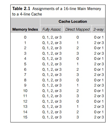
As an example, suppose our main memory consists
of 16 lines with indexes 0–15, and our cache consists of 4 lines with indexes
0–3. In a fully associative cache, line 0 can be assigned to cache location 0,
1, 2, or 3. In a direct mapped cache, we might assign lines by looking at their
remainder after division by 4. So lines 0, 4, 8, and 12 would be mapped to
cache index 0, lines 1, 5, 9, and 13 would be mapped to cache index 1, and so
on. In a two way set associative cache, we might group the cache into two sets:
indexes 0 and 1 form one set—set 0—and indexes 2 and 3 form another— set 1. So
we could use the remainder of the main memory index modulo 2, and cache line 0
would be mapped to either cache index 0 or cache index 1. See Table 2.1.
When more than one line in memory can be mapped
to several different locations in a cache (fully associative and n-way set associative), we also need to be able
to decide which line should be replaced or evicted. In our preceding example, if, for example, line 0 is in location
0 and line 2 is in location 1, where would we store line 4? The most commonly
used scheme is called least recently used. As the name suggests, the cache has a record
of the relative order in which the blocks have been
used, and if line 0 were used more recently
than line 2, then line 2 would be evicted and replaced by line 4.
3. Caches and programs: an example
It’s important to remember that the workings of
the CPU cache are controlled by the system hardware, and we, the programmers,
don’t directly determine which data and which instructions are in the cache.
However, knowing the principle of spatial and temporal locality allows us to
have some indirect control over caching. As an example, C stores
two-dimensional arrays in “row-major” order. That is, although we think of a
two-dimensional array as a rectangular block, memory is effectively a huge
one-dimensional array. So in row-major storage, we store row 0 first, then row
1, and so on. In the following two code segments, we would expect the first
pair of nested loops to have much better performance than the second, since
it’s accessing the data in the two-dimensional array in contiguous blocks.
double A[MAX][MAX], x[MAX], y[MAX];
. . .
/* Initialize A and x, assign y = 0 */
. . .
/* First pair of loops */
for (i =
0; i < MAX; i++)
for (j =
0; j < MAX; j++)
y[i] += A[i][j] x[j];
. . .
/* Assign y = 0 */
. . .
/* Second pair of loops */
for (j =
0; j < MAX; j++)
for (i =
0; i < MAX; i++)
y[i] += A[i][j] x[j];
To better understand this, suppose MAX is four, and the elements of A are stored in memory as follows:
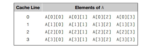
So, for example, A[0][1] is stored immediately after A[0][0] and A[1][0] is stored immediately after A[0][3].
Let’s suppose that none of the elements of A are in the cache when each pair of loops starts executing. Let’s
also suppose that a cache line consists of four elements of A and A[0][0] is the first element of a cache line. Finally,
we’ll suppose that the cache is direct mapped and it can only store eight
elements of A, or two cache lines. (We won’t worry about x and y.)
Both pairs of loops attempt to first access A[0][0]. Since it’s not in the cache, this will result in a cache miss,
and the system will read the line consisting of the first row of A, A[0][0], A[0][1], A[0][2], A[0][3], into the cache. The first pair of loops then accesses A[0][1], A[0][2], A[0][3], all of which are in the cache, and the next miss in the first
pair of loops will occur when the code accesses A[1][0]. Continuing in this fashion, we see that the
first pair of loops will result in a total of four misses when it accesses
elements of A, one for each row. Note that since our hypothetical cache can only
store two lines or eight elements of A, when we read the first element of row two and
the first element of row three, one of the lines that’s already in the cache
will have to be evicted from the cache, but once a line is evicted, the first
pair of loops won’t need to access the elements of that line again.
After reading the first row into the cache, the
second pair of loops needs to then access A[1][0], A[2][0], A[3][0], none of which are in the cache. So the next
three accesses of A will also result in misses. Furthermore,
because the cache is small, the reads of A[2][0] and A[3][0] will require that lines already in the cache
be evicted. Since A[2][0] is stored in cache line 2, reading its line
will evict line 0, and reading A[3][0] will evict line 1. After finishing the first
pass through the outer loop, we’ll next need to access A[0][1], which was evicted with the rest of the first row. So we see that every time we read an element of A, we’ll have a miss, and the second pair of loops results in 16
misses.
Thus, we’d expect the first pair of nested
loops to be much faster than the second. In fact, if we run the code on one of
our systems with MAX = 1000, the first pair of nested loops is
approximately three times faster than the second pair.
4. Virtual memory
Caches make it possible for the CPU to quickly
access instructions and data that are in main memory. However, if we run a very
large program or a program that accesses very large data sets, all of the
instructions and data may not fit into main memory. This is especially true
with multitasking operating systems; in order to switch between programs and
create the illusion that multiple programs are running simultaneously, the
instructions and data that will be used during the next time slice should be in
main memory. Thus, in a multitasking system, even if the main memory is very
large, many running programs must share the available main memory. Furthermore,
this sharing must be done in such a way that each program’s data and
instructions are protected from corruption by other programs.
Virtual memory was developed so that main memory can function
as a cache for secondary storage. It exploits the
principle of spatial and temporal locality by keeping in main memory only the
active parts of the many running programs; those parts that are idle are kept
in a block of secondary storage called swap space. Like
CPU caches, virtual memory operates on blocks
of data and instructions. These blocks are commonly called pages, and since secondary storage access can be
hun-dreds of thousands of times slower than main memory access, pages are
relatively large—most systems have a fixed page size that currently ranges from
4 to 16 kilobytes.
We may run into trouble if we try to assign
physical memory addresses to pages when we compile a program. If we do this,
then each page of the program can only be assigned to one block of memory, and
with a multitasking operating system, we’re likely to have many programs
wanting to use the same block of memory. In order to avoid this problem, when a
program is compiled, its pages are assigned virtual page numbers. Then, when the program is run, a table is created
that maps the vir-
tual page numbers to physical addresses. When
the program is run and it refers to a virtual address, this page table is used to translate the virtual address into
a physical address. If the creation of the page table is managed by the
operating system, it can ensure that the memory used by one program doesn’t
overlap the memory used by another.
A drawback to the use of a page table is that
it can double the time needed to access a location in main memory. Suppose, for
example, that we want to execute an instruction in main memory. Then our
executing program will have the virtual address of this instruction, but before we can find the
instruction in memory, we’ll need to translate the virtual address into a
physical address. In order to do this, we’ll need to find the page in memory
that contains the instruction. Now the vir-tual page number is stored as a part
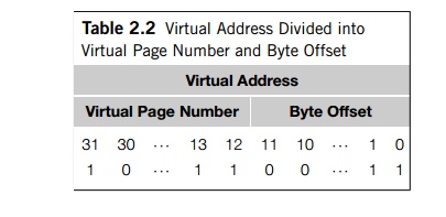
of the virtual address. As an example, suppose our addresses are 32 bits and
our pages are 4 kilobytes D 4096 bytes. Then each byte in the page can be
identified with 12 bits, since 212 D 4096. Thus, we can use the low-order 12 bits
of the virtual address to locate a byte within a page, and the remaining bits
of the virtual address can be used to locate an individual page. See Table 2.2.
Observe that the virtual page number can be computed from the virtual address
with-out going to memory. However, once we’ve found the virtual page number,
we’ll need to access the page table to translate it into a physical page. If
the required part of the page table isn’t in cache, we’ll need to load it from
memory. After it’s loaded, we can translate our virtual address to a physical
address and get the required instruction.
This is clearly a problem. Although multiple
programs can use main memory at more or less the same time, using a page table
has the potential to significantly increase each program’s overall run-time. In
order to address this issue, processors have a special address translation
cache called a translation-lookaside buffer, or TLB. It caches a small number of entries
(typically 16–512) from the page table in very fast memory. Using the principle
of spatial and temporal locality, we would expect that most of our memory
references will be to pages whose physical address is stored in the TLB, and
the number of memory references that require accesses to the page table in main
memory will be substantially reduced.
The terminology for the TLB is the same as the
terminology for caches. When we look for an address and the virtual page number
is in the TLB, it’s called a TLB hit. If it’s not in the TLB, it’s called a miss. The terminology for the page table, however, has an important
difference from the terminology for caches. If we attempt to access a page
that’s not in memory, that is, the page table doesn’t have a valid physical
address for the page and the page is only stored on disk, then the attempted
access is called a
page fault.
The relative slowness of disk accesses has a
couple of additional consequences for virtual memory. First, with CPU caches we
could handle write-misses with either a write-through or write-back scheme.
With virtual memory, however, disk accesses are so expensive that they should
be avoided whenever possible, so virtual memory always uses a write-back
scheme. This can be handled by keeping a bit on each page in memory that
indicates whether the page has been updated. If it has been updated, when it is
evicted from main memory, it will be written to disk. Second, since disk
accesses are so slow, management of the page table and the handling of disk
accesses can be done by the operating system. Thus, even though we as
programmers don’t directly control virtual memory, unlike CPU caches, which are
handled by system hardware, virtual memory is usually controlled by a
combination of system hardware and operating system software.
5. Instruction-level parallelism
Instruction-level parallelism, or ILP, attempts to improve processor
performance by having multiple processor components or functional units simultaneously exe-cuting instructions. There
are two main approaches to ILP: pipelining, in which functional units are arranged in stages, and multiple issue, in which multiple instruc-tions can be
simultaneously initiated. Both approaches are used in virtually all modern
CPUs.
Pipelining
The principle of pipelining is similar to a
factory assembly line: while one team is bolting a car’s engine to the chassis,
another team can connect the transmission to the engine and the driveshaft of a
car that’s already been processed by the first team, and a third team can bolt
the body to the chassis in a car that’s been processed by the first two teams.
As an example involving computation, suppose we want to add the floating point
numbers 9.87 104 and 6.54 103. Then we can use the
following steps:
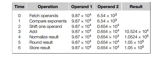
Here we’re using base 10 and a three digit
mantissa or significand with one digit to the left of the decimal point. Thus,
in the example, normalizing shifts the decimal point one unit to the left, and
rounding rounds to three digits.
Now if each of the operations takes one
nanosecond (10 9 seconds), the addition operation will take seven
nanoseconds. So if we execute the code
float x[1000],
y[1000], z[1000];
. . .
for (i =
0; i < 1000; i++)
z[i] = x[i] + y[i];
the for loop will take something like 7000 nanoseconds.
As an alternative, suppose we divide our
floating point adder into seven sepa-rate pieces of hardware or functional
units. The first unit will fetch two operands, the second will compare
exponents, and so on. Also suppose that the output of one functional unit is
the input to the next. So, for example, the output of the functional unit that
adds the two values is the input to the unit that normalizes the result. Then a
single floating point addition will still take seven nanoseconds. However, when
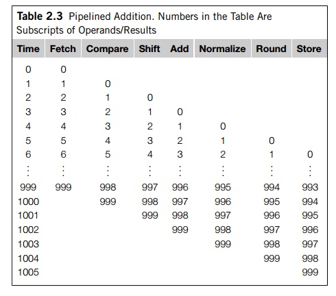
we execute the for loop, we can fetch x[1] and y[1] while we’re comparing the expo-nents of x[0] and y[0]. More generally, it’s possible for us to
simultaneously execute seven different stages in seven different additions. See
Table 2.3. From the table we see that after time 5, the pipelined loop produces
a result every nanosecond, instead of every seven nanoseconds, so the total
time to execute the for loop has been reduced from 7000 nanoseconds to 1006 nanoseconds—an
improvement of almost a factor of seven.
In general, a pipeline with k stages won’t get a k-fold improvement in per-formance. For example, if the times
required by the various functional units are different, then the stages will
effectively run at the speed of the slowest functional unit. Furthermore,
delays such as waiting for an operand to become available can cause the
pipeline to stall. See Exercise 2.1 for more details on the performance of
pipelines.
Multiple issue
Pipelines improve performance by taking
individual pieces of hardware or functional units and connecting them in
sequence. Multiple issue processors replicate functional units and try to
simultaneously execute different instructions in a program. For exam-ple, if we
have two complete floating point adders, we can approximately halve the time it
takes to execute the loop
for (i =
0; i < 1000; i++)
z[i] = x[i] + y[i];
While the first adder is computing z[0], the second can compute z[1]; while the first is computing z[2], the second can compute z[3]; and so on.
If the functional units are scheduled at
compile time, the multiple issue system is said to use static multiple issue. If they’re scheduled at
run-time, the system is said to use dynamic multiple issue. A processor that supports dynamic multiple issue
is sometimes said to be superscalar.
Of course, in order to make use of multiple
issue, the system must find instruc-tions that can be executed simultaneously.
One of the most important techniques is speculation. In speculation, the compiler or the processor makes a guess about
an instruction, and then executes the instruction
on the basis of the guess. As a sim-ple example, in the following code, the
system might predict that the outcome of z = x +
y will give z a positive value, and, as a consequence, it
will assign w = x.
z = x + y;
if (z > 0)
w = x;
else
w = y;
As another example, in the code
z = x + y;
w = a_p; /* a p is a pointer */
the system might predict that a_p does not refer to z, and hence it can simultaneously execute the
two assignments.
As both examples make clear, speculative
execution must allow for the possibility that the predicted behavior is
incorrect. In the first example, we will need to go back and execute the
assignment w = y if the assignment z = x + y results in a value that’s not positive. In the
second example, if a p does point to z, we’ll need to re-execute the assignment w = *a_p.
If the compiler does the speculation, it will
usually insert code that tests whether the speculation was correct, and, if
not, takes corrective action. If the hardware does the speculation, the
processor usually stores the result(s) of the speculative execution in a
buffer. When it’s known that the speculation was correct, the contents of the
buffer are transferred to registers or memory. If the speculation was
incorrect, the contents of the buffer are discarded and the instruction is
re-executed.
While dynamic multiple issue systems can
execute instructions out of order, in current generation systems the
instructions are still loaded in order and the results of the instructions are
also committed in order. That is, the results of instructions are written to
registers and memory in the program-specified order.
Optimizing compilers, on the other hand, can
reorder instructions. This, as we’ll see later, can have important consequences
for shared-memory programming.
6. Hardware multithreading
ILP can be very difficult to exploit: it is a
program with a long sequence of depen-dent statements offers few opportunities.
For example, in a direct calculation of the Fibonacci numbers
f[0] = f[1] = 1;
for (i =
2; i <= n; i++)
f[i] = f[i-1] + f[i-2];
there’s essentially no opportunity for
simultaneous execution of instructions. Thread-level parallelism, or TLP, attempts to provide parallelism
through the simultaneous execution of different threads, so it provides a coarser-grained parallelism than ILP, that is, the program
units that are being simultaneously executed—threads—are larger or coarser than
the finer-grained units—individual instructions.
Hardware multithreading provides a means for systems to continue doing
use-ful work when the task being currently executed has stalled—for example, if
the current task has to wait for data to be loaded from memory. Instead of
looking for parallelism in the currently executing thread, it may make sense to
simply run another thread. Of course, in order for this to be useful, the
system must support very rapid switching between threads. For example, in some
older systems, threads were sim-ply implemented as processes, and in the time
it took to switch between processes, thousands of instructions could be
executed.
In fine-grained multithreading, the processor switches between threads after each
instruction, skipping threads that are stalled. While this approach has the
potential to avoid wasted machine time due to stalls, it has the drawback that
a thread that’s ready to execute a long sequence of instructions may have to
wait to execute every instruction. Coarse-grained multithreading attempts to avoid this problem
by only switching threads that are stalled waiting for a time-consuming
operation to complete (e.g., a load from main memory). This has the virtue that
switching threads doesn’t need to be nearly instantaneous. However, the
processor can be idled on shorter stalls, and thread switching will also cause
delays.
Simultaneous multithreading, or SMT, is a variation on fine-grained
multi-threading. It attempts to exploit superscalar processors by allowing
multiple threads to make use of the multiple functional units. If we designate
“preferred” threads— threads that have many instructions ready to execute—we
can somewhat reduce the problem of thread slowdown.
Related Topics