Noise Characterisation

INTRODUCTION:

Noise is often described as the limiting factor in communication systems: indeed if there as no noise there would be virtually no problem in communications.

Noise is a general term which is used to describe an unwanted signal which affects a wanted signal. These unwanted signals arise from a variety of sources which may be considered in one of two main categories:-

a)     Interference, usually from a human source (manmade)

b)    Naturally occurring random noise.

Interference arises for example, from other communication systems (cross talk), 50 Hz supplies (hum) and harmonics, switched mode power supplies, thyristor circuits, ignition (car spark plugs) motors … etc. Interference can in principle be reduced or completely eliminated by careful engineering (i.e. good design, suppression, shielding etc). Interference is essentially deterministic (i.e. random, predictable), however observe.

When the interference is removed, there remains naturally occurring noise which is essentially random (non-deterministic),. Naturally occurring noise is inherently present in electronic communication systems from either ‗external‘ sources or ‗internal‘ sources.

Naturally occurring external noise sources include atmosphere disturbance (e.g. electric storms, lighting, ionospheric effect etc), so called ‘Sky Noise‘ or Cosmic noise which includes noise from galaxy, solar noise and ‗hot spot‘ due to oxygen and water vapour resonance in the earth‘s atmosphere. These sources can seriously affect all forms of radio transmission and the design of a radio system (i.e. radio, TV, satellite) must take these into account.The diagram below shows noise temperature (equivalent to noise power, we shall discuss later) as a function of frequency for sky noise.

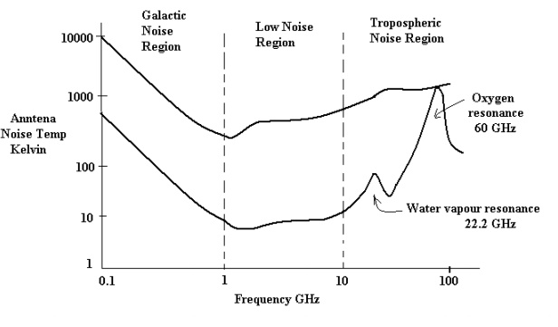
The upper curve represents an antenna at low elevation (~ 5^o above horizon), the lower curve represents an antenna pointing at the zenith (i.e. 90^o elevation).

Contributions to the above diagram are from galactic noise and atmospheric noise as shown below.Note that sky noise is least over the band – 1 GHz to 10 GHz. This is referred to as a low noise ‘window‘ or region and is the main reason why satellite links operate at frequencies in this band (e.g. 4 GHz, 6GHz, 8GHz). Since signals received from satellites are so small it is important to keep the background noise to a minimum.

Naturally occurring internal noise or circuit noise is due to active and passive electronic devices (e.g. resistors, transistors ...etc) found in communication systems. There are various mechanism which produce noise in devices; some of which will be discussed in the following sections.

·        THERMAL NOISE (JOHNSON NOISE):

This type of noise is generated by all resistances (e.g. a resistor, semiconductor, the resistance of a resonant circuit, i.e. the real part of the impedance, cable etc).

Free electrons are in contact random motion for any temperature above absolute zero (0 degree K, ~ -273 degree C). As the temperature increases, the random motion increases, hence thermal noise, and since moving electron constitute a current, although there is no net current flow, the motion can be measured as a mean square noise value across the resistance.

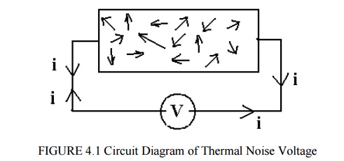
Experimental results (by Johnson) and theoretical studies (by Nyquist) give the mean square noise

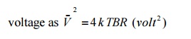
Where k = Boltzmann‘s constant = 1.38 x 10^-23 Joules per K

T = absolute temperature

B = bandwidth noise measured in (Hz)

R = resistance (ohms)

The law relating noise power, N, to the temperature and bandwidth is

N = k TB watts

These equations will be discussed further in later section.

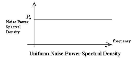
The equations above held for frequencies up to > 10¹³ Hz (10,000 GHz) and for at least all practical temperatures, i.e. for all practical communication systems they may be assumed to be valid.Thermal noise is often referred to as ‘white noise‘ because it has a uniform ‘spectral density‘.

Note – noise power spectral density is the noise power measured in a 1 Hz bandwidth i.e. watts per Hz. A uniform spectral density means that if we measured the thermal noise in any 1 Hz bandwidth from ~ 0Hz → 1 MHz → 1GHz …….. 10,000 GHz etc we would measure the same amount of noise.

From the equation N=kTB, noise power spectral density is p_o = k T watts per Hz. I.e. Graphically figure 4.2 is shown as,

·        SHOT NOISE:

Shot noise was originally used to describe noise due to random fluctuations in electron emission from cathodes in vacuum tubes (called shot noise by analogy with lead shot). Shot noise also occurs in semiconductors due to the liberation of charge carriers, which have discrete amount of charge, in to potential barrier region such as occur in pn junctions. The discrete amounts of charge give rise to a current which is effectively a series of current pulses.

For pn junctions the mean square shot noise current is

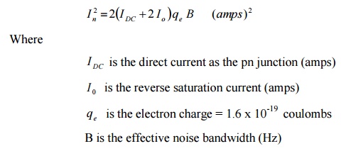
Shot noise is found to have a uniform spectral density as for thermal noise.

·        LOW FREQUENCY OR FLICKER NOISE:

Active devices, integrated circuit, diodes, transistors etc also exhibits a low frequency noise, which is frequency dependent (i.e. non uniform) known as flicker noise or ‘one – over – f‘ noise.

The mean square value is found to be proportional to  (1/f) where f is the frequency and n= 1. 

Thus the noise at higher frequencies is less than at lower frequencies. Flicker noise is due to impurities in the material which in turn cause charge carrier fluctuations.

·        EXCESS RESISTOR NOISE:

Thermal noise in resistors does not vary with frequency, as previously noted, by many resistors also generates as additional frequency dependent noise referred to as excess noise. This noise also exhibits a (1/f) characteristic, similar to flicker noise.

Carbon resistor generally generates most excess noise whereas were wound resistors usually generates negligible amount of excess noise. However the inductance of wire wound resistor limits their frequency and metal film resistor are usually the best choices for high frequency communication circuit where low noise and constant resistance are required.

·        BURST NOISE OR POPCORN NOISE:

Some semiconductors  also  produce  burst or popcorn noise  with a  spectral  density which  is proportional to (1/f)2

^ü   GENERAL COMMENTS:

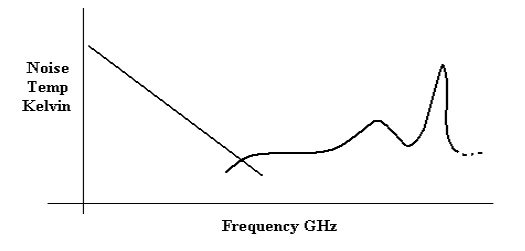
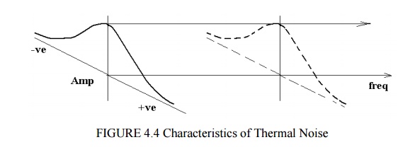
The diagram below illustrates the variation of noise with frequency.

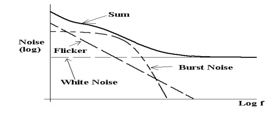
For frequencies below a few KHz (low frequency systems), flicker and popcorn noise are the most significant, but these may be ignored at higher frequencies where ‗white‘ noise predominates.

Thermal noise is always presents in electronic systems. Shot noise is more or less significant depending upon the specific devices used for example as FET with an insulated gate avoids junction shot noise. As noted in the preceding discussion, all transistors generate other types of

‗non-white‘ noise which may or may not be significant depending on the specific device and application. Of all these types of noise source, white noise is generally assumed to be the most significant and system analysis is based on the assumption of thermal noise. This assumption is reasonably valid for radio systems which operates at frequencies where non-white noise is greatly reduced and which have low noise ‗front ends‘ which, as shall be discussed, contribute most of the internal (circuit) noise in a receiver system. At radio frequencies the sky noise contribution is significant and is also (usually) taken into account.

Obviously, analysis and calculations only gives an indication of system performance. Measurements of the noise or signal-to-noise ratio in a system include all the noise, from whatever source, present at the time of measurement and within the constraints of the measurements or system bandwidth.

Before discussing some of these aspects further an overview of noise evaluation as applicable to communication systems will first be presented.

^ü   NOISE EVALUATION:

·        OVERVIEW:

It has been stated that noise is an unwanted signal that accompanies a wanted signal, and, as discussed, the most common form is random (non-deterministic) thermal noise.

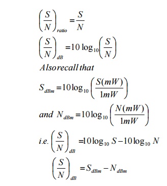
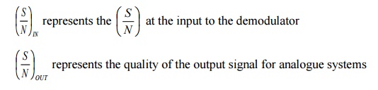
The essence of calculations and measurements is to determine the signal power to Noise power ratio, i.e. the (S/N) ratio or (S/N) expression in dB.

i.e. Let S= signal power (mW) 

N = noise power (mW)

Noise, which accompanies the signal is usually considered to be additive (in terms of powers) and its often described as Additive White Gaussian Noise, AWGN, noise. Noise and signals may also Powers are usually measured in dBm (or dBw) in communications systems. The equation (S/N)dB = SdBM - NdBm is often the most useul. The (S/N) at various stages in a communication system gives an indication of system quality and  performance in terms of error rate in digital data communication systems and ‗fidelity‘ in case of analogue communication systems. (Obviously, the larger the (S/N) , the better the system will be).

AWGN.In order to evaluate noise various mathematical models and techniques have to be used, particularly concepts from statistics and probability theory, the major starting point being that random noise is assumed to have a Gaussian or Normal distribution.

We may relate the concept of white noise with a Gaussian distribution as follows:

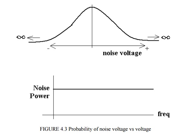
Gaussian distribution – ‗graph‘ shows Probability of noise voltage vs voltage – i.e. most probable noise voltage is 0 volts (zero mean). There is a small probability of very large +ve or –ve noise voltages.

White noise – uniform noise power from ‘DC‘ to very high frequencies.

Although not strictly consistence, we may relate these two characteristics of thermal noise as follows:

The probability of amplitude of noise at any frequency or in any band of frequencies (e.g. 1 Hz, 10Hz… 100 KHz .etc) is a Gaussian distribution.Noise may be quantified in terms of noise power spectral density, p₀ watts per Hz, from which Noise power N may be expressed as

N= p₀ B_n watts

Where B_n is the equivalent noise bandwidth, the equation assumes p₀ is constant across the band (i.e. White Noise).

Note - B_n is not the 3dB bandwidth, it is the bandwidth which when multiplied by p₀

Gives the actual output noise power N. This is illustrated further below.

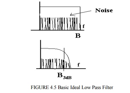
Ideal low pass filter

             Bandwidth B Hz = B_n

             N= p₀ B_n watts

Practical LPF

             3 dB bandwidth shown, but noise does not suddenly cease at B_3dB

             Therefore, B_n > B_3dB, B_n depends on actual filter.

             N= p₀ B_n

In general the equivalent noise bandwidth is > B_3dB.

Alternatively, noise may be quantified in terms of ‘mean square noise‘ i.e. bar (V²) , which is effectively a power. From this a ‗Root mean square (RMS)‘ value for the noise voltage may be determined.

In order to ease analysis, models based on the above quantities are used. For example, if we imagine noise in a very narrow bandwidth, δf, as δf->df, the noise approaches a sine wave (with frequency ‘centred‘ in df).Since an RMS noise voltage can be determined, a ‗peak‘ value of the noise may be invented since for a sine wave

Note – the peak value is entirely fictious since in theory the noise with a Gaussian distribution could have a peak value of + ¥ or - ¥ volts.

Hence we may relate

Problems arising from noise are manifested at the receiving end of a system and hence most of the analysis relates to the receiver / demodulator with transmission path loss and external noise sources (e.g. sky noise) if appropriate, taken into account.

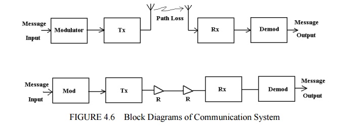
Transmission Line

R = repeater (Analogue) or Regenerators (digital)

These systems may facilitate analogue or digital data transfer. The diagram below characterizes these typical systems in terms of the main parameters.

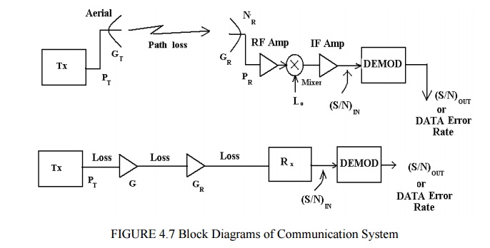
PT represents the output power at the transmitter. transmitter. 

G_T represents the Tx aerial gain.

Path loss represents the signal attenuation due to inverse square law and absorption e.g. in atmosphere.

G represents repeater gains.

P_R represents receiver inout signal power

N_R represents the received external noise (e.g. sky noise)

G_R represents the receiving aerial gain.

^ü   DATA ERROR RATE represents the quality of the output (probability of error) for

digital data system.